pkg <- function(x, ...) {
  if (knitr::is_html_output()) {
    paste0("**", x, "**")
  } else {
    paste0(r"(\pkg{)", x, r"(\})")
  }
}
In [1]:
In [2]:
remotes::install_github("swang87/bcp")In [3]:
manual <- c("tsibble", "tibble", "changepoint", "ggchangepoint", "wbs", "qcc", "GA", "stats", "ecp", "changepoint.np", "purrr", "bcp", "mcp", "tidychangepoint", "EnvCpt", "tsibbledata", "broom", "strucchange", "changepointGA", "segmented", "pkgsearch")
pkgs <- unique(c(manual, .packages()))
knitr::write_bib(pkgs, file = "pkgs.bib")
Warning in xfun::pkg_bib(..., prefix = prefix): package(s) bcp not found1 Introduction
1.1 Motivation
While global temperatures continue to rise, climate scientists continue to face baffling skepticism from some. How do we know that the increases we observe are not just anecdotal? How do we know that the recent pattern of rising temperatures is not simply the latest round of normal fluctuation?
One approach would be to measure temperature over a long period of time, and investigate the time series for the presence of changepoints. Changepoints indicate breaks in a time series that divide it into mutually exclusive regions in which the behavior of the underlying system is the same within each region, but varies across regions. A changepoint might represent a moment at which the system changed in some meaningful and measurable way.
Changepoint detection analysis is the study of such changepoints and the algorithms and models that determine them. Unfortunately, there is no known general solution to the Changepoint Detection Problem (CDP, defined formally in Section 1.4). Furthermore—and more germaine for us—the objects returned by changepoint detection functions from various R packages (see Section 1.6) are all of different types, have different structures, contain different information, and can be used with a variety of different functions. This heterogeneity in user interface and package architecture is widespread across roughly a dozen other changepoint detection packages we found (see Section 1.6). No standardization exists.
These incompatible software interfaces make it unnecessarily difficult to compare the performance of changepoint detection algorithms across different packages. One essentially has to write custom code for each implementation, even when using the same data set. Furthermore, since there is no pre-built interface for genetic changepoint detection algorithms, every tweak to a genetic algorithm for changepoint detection requires custom code.
While we do not claim to offer solutions to the CDP itself, tidychangepoint solves the software heterogeneity problem by providing a unified interface with built-in support for genetic algorithms for changepoint detection. Comparing algorithms and/or models for changepoint detection in tidychangepoint can be as easy as iterating over a list of specifications (see Section 1.3).
1.2 An example illustrating the status quo
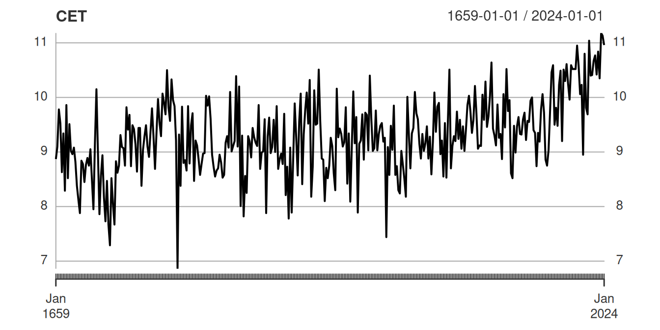
For example, the CET data set collected by Parker, Legg, and Folland (1992) and repackaged in tidychangepoint (Baumer et al. 2026) lists the mean annual temperature in degrees Celsius from 1659 to 2024, as measured in Central England and shown in Figure 1. When did the temperature start to rise? How can we distinguish natural variation in temperature (around a static mean) from a meaningful change in that mean (caused by humans)?
In [4]:
Suppose that you are interested in determining changepoints for the CET data set, but you don’t know much about the inner workings of changepoint detection algorithms. You decide to simply fit a bunch of off-the-shelf changepoint detection models and compare the results. Some googling leads you to four packages: strucchange (Zeileis et al. 2024), segmented (V. M. R. Muggeo 2026), changepoint (Killick 2024), and wbs (Baranowski and Fryzlewicz 2024).
First, you fit four models. Note that because CET is an xts object, sometimes (but not always), you have to cast it to a ts object.
In [5]:
cet_cpt <- changepoint::cpt.meanvar(as.ts(CET))
cet_wbs <- wbs::wbs(CET)
cet_bkp <- strucchange::breakpoints(CET ~ 1)
cet_seg <- segmented::stelpmented(as.ts(CET))
Next, you seek to recover the changepoints as a numeric vector. These are the indices of the time series (in this case, each corresponds to a year since 1659). Note that each object (some of which are S3 and some of which are S4) stores the changepoints in different locations, some of which are not easy to find.
In [6]:
cet_cpt@cpts[1] 55 57 267 344 347 366sort(cet_wbs$cpt$cpt.ic$mbic.penalty)[1] 43 252 330cet_bkp$breakpoints[1] 55 252 312cet_seg$psi[ , 1] psi1.id psi2.id psi3.id
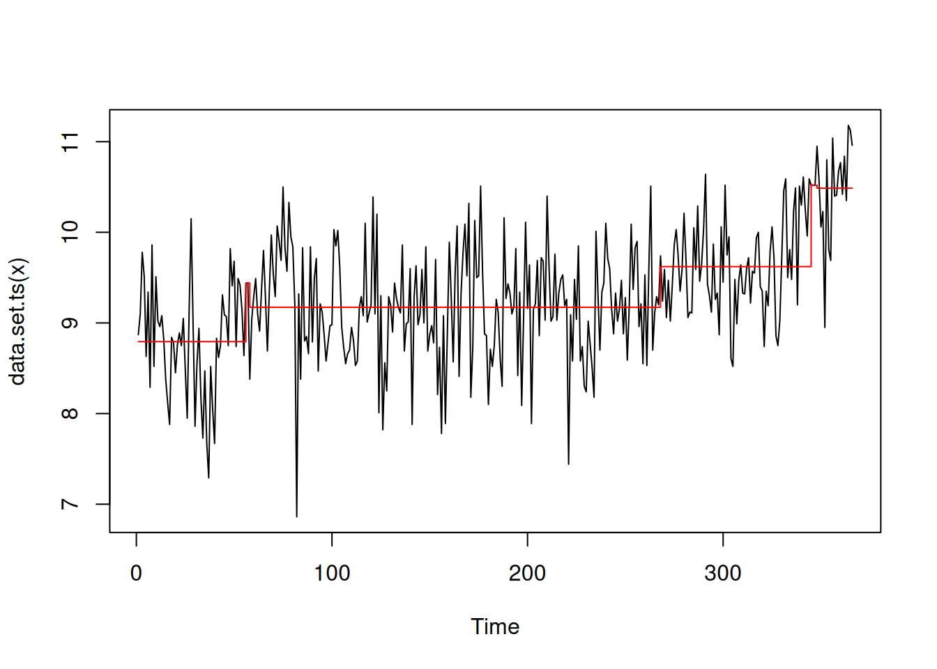
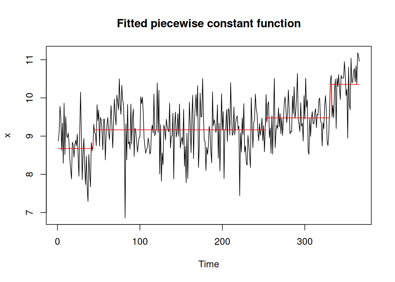
43.25624 267.24343 338.92795 Finally, you plot each object using plot(). Figure 11 in our Appendix shows the resulting plots, some of which add changepoints and model estimates to the original time series, and others of which show diagnostic plots.
While you were able to conduct your analysis, you had to learn the ins-and-outs of four different packages, all of which were designed in their own way.
1.3 An example using tidychangepoint
tidychangepoint makes the comparisons in the previous section simpler by employing a unified syntax and output object. With tidychangepoint, it is possible to iterate analyses over lists of specifications.
We demonstrate this approach using the same four models as above, plus a null model that finds no changepoints, and a genetic algorithm that Shi et al. (2022) use to explore a variety of different parametric models using genetic algorithms and a previous version of the CET data set.1 Using a trendshift model (see Section 5), they identified the years 1700, 1739, and 1988 as changepoints.2.
In [7]:
library(tidyverse)── Attaching core tidyverse packages ──────────────────────── tidyverse 2.0.0 ──
✔ dplyr 1.2.0 ✔ readr 2.2.0
✔ forcats 1.0.1 ✔ stringr 1.6.0
✔ ggplot2 4.0.2 ✔ tibble 3.3.1
✔ lubridate 1.9.5 ✔ tidyr 1.3.2
✔ purrr 1.2.1
── Conflicts ────────────────────────────────────────── tidyverse_conflicts() ──
✖ dplyr::filter() masks stats::filter()
✖ dplyr::lag() masks stats::lag()
ℹ Use the conflicted package (<http://conflicted.r-lib.org/>) to force all conflicts to become errorsIn [8]:
cet_objs <- list(
  null = segment(CET, method = "null"),
  pelt = segment(CET, method = "pelt"),
  wbs = segment(CET, method = "wbs"),
  bkp = segment(CET, method = "strucchange"),
  seg = segment(CET, method = "stelpmented"),
  shi = segment(CET, method = "ga-shi", maxiter = 1000, run = 100)
)
In [9]:
cet_objs <- write_rds(cet_objs, here::here("cet_objs.rds"))In [10]:
cet_objs <- read_rds(here::here("cet_objs.rds"))Once the algorithms have been run, we can easily extract the sets of changepoints for comparison using the changepoints() function and convert them to human-interpretable years with the as_year() function.
In [11]:
cet_objs |>
  lapply(changepoints, use_labels = TRUE) |>
  lapply(as_year)
$null
character(0)
$pelt
[1] "1713" "1715" "1925" "2002" "2005"
$wbs
[1] "1701" "1739" "1740" "1892" "1988"
$bkp
[1] "1713" "1910" "1970"
$seg
[1] "1701" "1925" "1997"
$shi
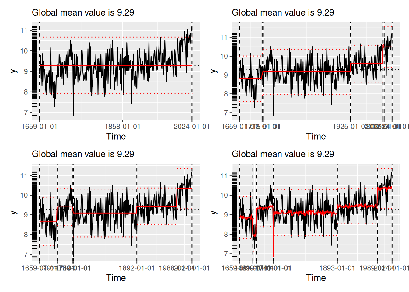
[1] "1691" "1699" "1740" "1741" "1893" "1989"We compare the results visually using plot() (see Figure 2), which now always situates the model estimates in the domain of the original time series. Each panel of Figure 2 shows the original time series (black line) segmented by the changepoints determined by the various algorithms (vertical dotted lines). The horizontal red lines indicate the mean and 1.96 times the standard deviation within each region, as per the summary produced by tidy() (see Section 3.2).
In [12]:
cet_objs |>
  lapply(plot, use_time_index = TRUE, ylab = "Degrees Celsius") |>
  patchwork::wrap_plots()
Scale for x is already present.
Adding another scale for x, which will replace the existing scale.
Scale for x is already present.
Adding another scale for x, which will replace the existing scale.
Scale for x is already present.
Adding another scale for x, which will replace the existing scale.
Scale for x is already present.
Adding another scale for x, which will replace the existing scale.
Scale for x is already present.
Adding another scale for x, which will replace the existing scale.
Scale for x is already present.
Adding another scale for x, which will replace the existing scale.Warning: Removed 1 row containing missing values or values outside the scale range
(`geom_segment()`).
Removed 1 row containing missing values or values outside the scale range
(`geom_segment()`).
Removed 1 row containing missing values or values outside the scale range
(`geom_segment()`).
Removed 1 row containing missing values or values outside the scale range
(`geom_segment()`).strucchange (lower-left), stelpmented (lower-middle), and Shi’s algorithm (lower-right). Note that the model in the lower-right panel includes an autoregressive parameter, and thus the model estimates vary across years within regions. All plots created by plot.tidycpt().
We return to this example in Section 2.1.
1.4 Mathematical problem formulation
Let \(y = \{y_1, \ldots, y_n\} \in \mathbb{R}^n\) be a discrete series of observations made over an integer-valued index of time points \(t = 1, \ldots, n\). Define \(\tau = \{\tau_1, \ldots, \tau_m\} \in [1,n]^m\) to be a set of time point indexes known as changepoints, for some \(0 \leq m \leq n\). The \(m\) changepoints divide the time series into \(m+1\) regions, with the idea that the behavior of the time series within each region does not change, and the changepoints represent points in time at which the behavior of the underlying system changes in some meaningful way. If we adopt the convention that \(\tau_0 = 1\) and \(\tau_{m+1} = n+1\) then the union of the set of half-open intervals \([\tau_j, \tau_{j+1})\) for \(0 \leq j \leq m\) covers the time domain of the series \(y\).
Even if the changepoints are assumed to come from the discrete set \(t\), there are (at least) \(2^n\) possible changepoint sets, and the Changepoint Detection Problem (CDP)—which is the problem of finding the optimal changepoint set (according to some metric)—has attracted considerable attention in the literature. Aminikhanghahi and Cook (2017) provide an excellent survey of relevant results. In the typical unsupervised setting in which the true changepoints are not known, various models, metrics, and algorithms to find the optimal changepoint set have been proposed, some of which are in widespread use. We briefly highlight the previous work most relevant to ours in Section 1.5, and review existing software implementations of these algorithms in Section 1.6. In any case, all attempts to solve the CDP considered in this paper involve three essential components: 1) a parametric model \(M(y | \theta)\) that describes the data-generating process of the time series; 2) an algorithm \(A\) to search the exponentially large space of possible changepoint sets; and 3) a metric \(f : (\tau, M) \rightarrow \mathbb{R}\) (a penalized objective function) for evaluating the suitability of any given changepoint set. We define \(\tau_{f, M, \theta}^*\) to be the changepoint set that minimizes the value of the penalized objective function \(f\) on the model \(M\) with parameters \(\theta\) over the space of all possible changepoint sets. That is, \[ \tau_{f, M, \theta_\tau}^* = \arg\min_{\tau \in [1,n]^m} f(\tau, M(y | \theta_\tau)) \] The value of the penalized objective function \(f(\tau, M(y|\hat{\theta}_\tau))\) is often referred to as the fitness of the changepoint set \(\tau\) and the model \(M\) with estimated parameters \(\hat{\theta}_\tau\) to the time series \(y\). Note that the value of the parameters \(\theta\) depend on the changepoint set \(\tau\), so we may write \(\theta_\tau\).
For example, perhaps the simplest and most common parametric model for changepoint detection is the normal (Gaussian) meanshift model, in which the time series \(y\) is assumed to be generated by a different random variable \(Y_j \sim \mathcal{N}(\mu_j, \sigma^2)\) for each region \(1 \leq j \leq m+1\). Thus the series mean \(\mu_j\) is constant within each of the \(m+1\) regions, but varies across the regions (piecewise stationarity), while the variance \(\sigma^2\) is constant over the entire time series. We fit the normal meanshift model using Maximium Likelihood Estimation (MLE), resulting in the estimated parameters \(\hat{\theta}_\tau = \{ \hat{\sigma}^2, m, \hat{\mu}_0, \ldots, \hat{\mu}_m \}\). If we choose the Bayesian Information Criterion (BIC) (Schwarz 1978) as our penalty, then the penalized objective function becomes: \[ BIC(\tau, M(y|\hat{\theta}_\tau)) = k_M(\tau) \ln{n} - 2 \ln{L_M(y | \hat{\theta}_\tau)}, \] where \(k_M(\tau)\) is the number of parameters estimated by the model (in this case, \(m + 3\), for \(m\), the \(m+1\) means, and the common standard deviation) and \(L_M(y|\hat{\theta}_\tau)\) is the likelihood function for \(M\), which in this case is (see S. Li and Lund (2012) for details): \[ L_M(y|\hat{\theta}_\tau) = -\frac{n}{2}(\ln{\hat{\sigma}^2} + 1 + \ln{2 \pi}) \,. \]
In general, while the true value of \(\tau_{BIC, meanshift, \hat{\theta}}^*\) is unknown, under reasonable assumptions about the growth of the penalized objective function with respect to the number of changepoints, the PELT algorithm (Killick, Fearnhead, and Eckley 2012) will find the exact value in polynomial time.
More generally, given a time series \(y\), a parametric model \(M(y|\theta)\), and a penalized objective function \(f\), the goal of any changepoint detection algorithm \(A\) is to search the exponentially large space of possible changepoints sets for the one \(\tau^*\) that minimizes the value of \(f(\tau, M(y|\hat{\theta}_\tau))\). Of course, in the process it must also estimate \(\hat{\theta}_\tau\).
1.5 Selected changepoint detection algorithms
Aminikhanghahi and Cook (2017) provide a comprehensive survey of different models for changepoint detection in time series. This includes classifications of offline vs. online algorithms, supervised vs. unsupervised problems, computational concerns, robustness, open problems, and the distribution of changepoints within long time series. Guédon (2015) quantifies the uncertainty in the segmentation of diverse sets of changepoints, using both Bayesian and non-Bayesian techniques.
The Pruned Exact Linear Time (PELT) algorithm developed by Killick, Fearnhead, and Eckley (2012) builds on a dynamic programming algorithm from Jackson et al. (2005) to offer a linear time, exact algorithm for changepoint detection. PELT offers order of magnitude improvements in computational cost (i.e., \(O(n)\) vs. the \(O(n \log{n})\) performance of the binary segmentation algorithm (Scott and Knott 1974) and the \(O(n^3)\) performance of the segmented neighborhood algorithm (Auger and Lawrence 1989)), and is capable of optimizing over different parametric models (e.g., meanvar, meanshift, etc.) and different penalized objective functions (e.g., BIC, MBIC (see Section 6.1.2), etc.). To guarantee an optimal solution, PELT requires that the value of the penalized objective function decreases (or increases by an amount bounded by a known constant) with each additional changepoint. Moreover, its running time can be quadratic (i.e., \(O(n^2)\)) unless the number of changepoints grows linearly with the length of the time series. While these assumptions are mild, not all possible combinations of time series, models, and penalty functions will meet them.3
S. Li and Lund (2012) illustrate how a genetic algorithm can provide good results by employing Darwinian principles (e.g., survival of the fittest) to search the space of all possible changepoint sets intelligently. For a given parametric model and penalized objective function, a genetic algorithm starts with an initial “generation” of (usually randomly generated) candidate changepoint sets, evaluates them all using the penalized objective function, then probabilistically “mates” the most promising candidate changepoint sets to produce a new generation of the same size. This process is repeated until a stopping criteria is met, and the single best (fittest) changepoint set is returned. While genetic algorithms are neither exact, nor deterministic, nor computationally efficient, they are more easily generalizable than PELT, and can return competitive results in practice (Shi et al. 2022). S. Li and Lund (2012) also develop the notion of the Minimum Descriptive Length (MDL) as a penalty function based on information theory.
Bai and Perron (1998) use linear regression models fit by least squares to detect changepoints. In particular, they construct a framework for testing the alternative hypothesis that there is one additional changepoint. Zeileis et al. (2003) build on this and related work by Bai and Perron (2003), using a series of F-statistics and a dynamic programming algorithm to find the set of changepoints that minimize the residual sum of squared errors (see Section 1.6). V. M. Muggeo (2003) also employs a linear regression framework, using the Davies test (Davies 1987) as criterion for a single changepoint and BIC as criterion for multiple changepoints (V. M. Muggeo et al. 2008).
Barry and Hartigan (1993) employ Bayesian techniques for changepoint detection. Cho and Fryzlewicz (2015) propose the Sparsified Binary Segmentation (SBS) algorithm, which uses CUSUM statistics to analyze high dimensional time series. This algorithm uses the concept of a threshold above which statistics are kept—an idea that resurfaces in Suárez-Sierra, Coen, and Taimal (2023). Cho (2016) explores the utility of a double CUSUM statistic for panel data. Hocking et al. (2013) use machine learning techniques to determine the optimal number of changepoints.
Suárez-Sierra, Coen, and Taimal (2023) detail the implementation of a changepoint detection heuristic we rebrand as Coen’s algorithm in this paper. Coen’s algorithm (Section 4.3) is genetic and uses a non-homogeneous Poisson process model (Section 5.3) to model the exceedances of a threshold over time, and a Bayesian Minimum Descriptive Length (BMDL, Section 6.1.4) penalized objective function. Taimal, Suárez-Sierra, and Rivera (2023) discuss modifications and performance characteristics of Coen’s algorithm.
1.6 Existing changepoint detection R packages
There are dozens of changepoint packages on CRAN, all of which have their strengths and limitations. Please see the “Comparison to other packages” vignette in the mcp (Lindeløv 2024) documentation for a thorough comparison.
In [13]:
pkgsearch::pkg_search(query = "changepoint|strucchange", size = 50) |>
  arrange(desc(downloads_last_month)) |>
  filter(downloads_last_month > 1000, revdeps > 2) |>
  select(package, revdeps, downloads_last_month, title) |>
  print(n = 50)
According to statistics returned by the pkgsearch (Csárdi and Salmon 2025) package, only three changepoint detection packages have more than 1000 downloads per month and more than two reverse dependencies: strucchange (Zeileis et al. 2024), segmented (V. M. R. Muggeo 2026), and changepoint (Killick 2024; Killick and Eckley 2014). tidychangepoint now supports all three.
strucchange (Zeileis et al. 2024, 2002) uses a regression-based framework and implements a dynamic programming algorithm to identify changepoints. The segmented (V. M. R. Muggeo 2026) package iteratively searches for optimal changepoint sets in a linear regression framework.
changepoint (Killick 2024; Killick and Eckley 2014) implements the algorithms PELT, Binary Segmentation, and Segmented Neighborhood. PELT employs one of three different models: meanshift, meanvar, and varshift (see Section 5). For the meanvar model (the most versatile) the data-generating model can follow a Normal, Poisson, Gamma, or Exponential distribution. Penalty functions (see Section 6) implemented by PELT include AIC, BIC, and MBIC, but not MDL. EnvCpt (Killick et al. 2025) is another package that wraps changepoint functionality.
The wbs (Baranowski and Fryzlewicz 2024) package implements the Wild Binary Segmentation and standard Binary Segmentation algorithms, the first of which is incorporated into tidychangepoint. The ggchangepoint (Yu 2022) package provides some wrapper functions and graphical tools for changepoint detection analysis that are similar to ours, but more limited in scope and usability. Nonparametric methods for changepoint detection are present in the ecp (James, Zhang, and Matteson 2024) and changepoint.np (Haynes and Killick 2022) packages. We consider these beyond our scope at this time, which is focused on parameteric models for changepoint detection.
A Bayesian approach is implemented in the bcp (R-bcp?; Erdman and Emerson 2008) package, which is no longer available on CRAN. The qcc (Scrucca 2017) package is more broadly focused on quality control and statistical process control, neither of which are specific to changepoint detection. The mcp (Lindeløv 2024) package focuses on regression-based, Bayesian methods.
The changepointGA (M. Li and Lu 2025) package appeared on CRAN subsequent to the submission of this paper. It provides a detailed implementation of several changepoint detection algorithms that are built on top of a custom algorithmic implementation (M. Li and Lu 2024). Note that in contrast, tidychangepoint relies on a more general-purpose genetic algorithm from the GA (Scrucca 2026) package as a backend. We have included basic support for the ARIMA model with a BIC penalty function in tidychangepoint.
1.7 Our contribution
In this paper, we present several substantive improvements to the existing state-of-the-art. First, the tidychangepoint package (Baumer et al. 2026) provides a unified interface that makes working with existing changepoint detection algorithms in a tidyverse-compliant syntax easy (Section 3). This reduces friction for anyone who wants to compare the results of algorithms, models, or penalized objective functions across different packages. Second, the architecture of the package is easily extended to incorporate new changepoint detection algorithms (Section 4), new parametric models (Section 5), and new penalized objective functions (Section 6). Indeed, our careful separation of these three essential elements of changepoint detection is in and of itself clarifying. Third, to the best of our knowledge, tidychangepoint is the first R package that allows users to run genetic algorithms for changepoint detection without having to write custom code. With GA as a backend, tidychangepoint provides a user-friendly interface for mixing-and-matching various parametric models, penalized objective functions, and initial populations in ways that previously required non-trivial programming by the user. Since tidychangepoint wraps functionality from other packages it adds only modest computational overhead, and delivers correct results (Section 7). Finally, tidychangepoint includes new or updated data sets packaged as time series objects about particulate matter in Bogotá, monthly rainfall in Medellín, temperature in Central England, and batting performance in Major League Baseball. We illustrate the utility of the package in Section 2 and conclude in Section 8.
tidychangepoint is available via download from the Comprehensive R Archive Network (CRAN) since August 19, 2024. The package website contains several short articles demonstrating how to use various features of the package, some of which are not included in this paper (for brevity).
2 Examples using tidychangepoint
In this Section we provide more detailed examples of how tidychangepoint can facilitate meaningful comparisons across algorithms, models, and penalized objective functions.
2.1 Temperatures in Central England
In Section 1.3, we noted that the comparative analysis across different models presented in Shi et al. (2022) required writing custom code for each model fit. In Section 5, we list the many parametric models that tidychangepoint includes. These include the “meanshift” (i.e., piecewise-constant) and “trendshift” (i.e., piecewise-linear) models, either of which can include AR(1) lagged errors, and either of which can be fit using the BIC or MDL penalties (see Section 6).
With tidychangepoint, we can employ a machine learning style approach to finding the best combination of model and penalty function for a time series. In this case, we build a data.frame with 8 possible combinations.
In [14]:
cet_options <- expand_grid(
  model_fn = c(fit_meanshift_norm, fit_meanshift_norm_ar1,
               fit_trendshift, fit_trendshift_ar1),
  penalty_fn = c(BIC, MDL)
)
Next, using functionality4 from the purrr package (Wickham and Henry 2026), we simply iterate the segment() function—which is the main workhorse in tidychangepoint—over these combinations. In each case we employ a genetic algorithm that can produce up to 5000 generations (maxiter), although it will stop if there is no improvement in the fitness (i.e., the value of the penalized objective function) after 100 consecutive generations (run).
In [15]:
library(purrr)
cet_mods <- cet_options |>
  mutate(
    tidycpt = map2(
      model_fn, penalty_fn, .f = segment,
      x = CET, method = "ga", maxiter = 5000, run = 100
    )
  )
In [16]:
cet_mods <- write_rds(cet_mods, here::here("cet_mods.rds"))In [17]:
library(purrr)
cet_mods <- read_rds(here::here("cet_mods.rds"))
The fitness(), changepoints() and model_name() functions can recover useful information from the resulting objects (see Section 3.2).
In [18]:
cet_mods <- cet_mods |>
  mutate(
    fitness = map_dbl(tidycpt, fitness),
    penalty = map_chr(tidycpt, ~names(fitness(.x))),
    num_cpts = map_int(tidycpt, ~length(changepoints(.x))),
    model_name = map_chr(tidycpt, model_name),,
    num_gens = map_int(tidycpt, ~nrow(as.segmenter(.x)@summary))
  )
We can now easily compare the results and learn about which model performed best with which penalty function.
In [19]:
cet_mods |>
  arrange(penalty, fitness) |>
  select(model_name, fitness, penalty, num_cpts, num_gens)
# A tibble: 8 × 5
model_name fitness penalty num_cpts num_gens
<chr> <dbl> <chr> <int> <int>
1 trendshift 671. BIC 3 1246
2 meanshift_norm_ar1 674. BIC 6 1362
3 meanshift_norm 680. BIC 9 1415
4 trendshift_ar1 682. BIC 4 1347
5 trendshift_ar1 662. MDL 5 2987
6 meanshift_norm 680. MDL 8 1480
7 meanshift_norm_ar1 683. MDL 5 1451
8 trendshift 702. MDL 9 1754In this case, the trendshift model with white noise errors produces the best fitness score with the BIC penalty, while adding AR(1) errors produces the best fitness score with the MDL penalty. These results accord with the findings by Shi et al. (2022).
2.2 The designated hitter in Major League Baseball
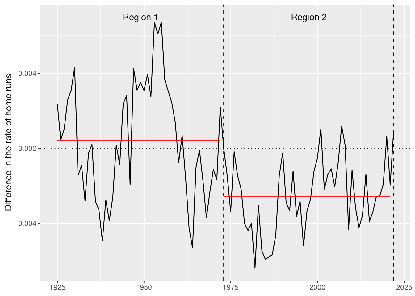
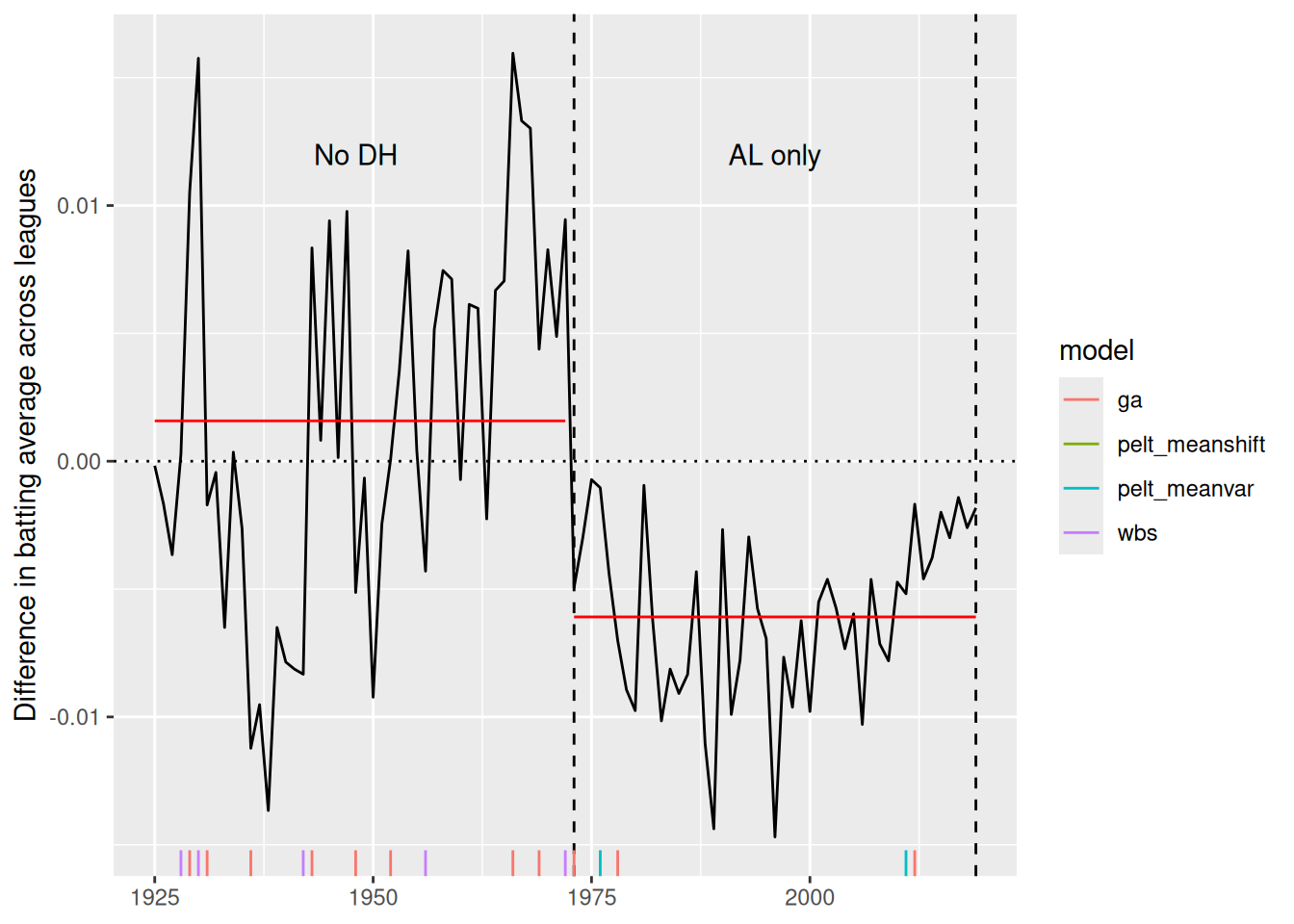
Sometimes we know the truth about when changepoints occur. For example, Figure 3 shows the difference in batting average between the American and National Leagues of Major League Baseball (MLB) from 1925–2019. The introduction of the designated hitter rule in the American League in 1973 led to noticeable differences in batting performance relative to the National League (which did not adapt the rule until 2020), because the rule allowed teams in the American League to designate another player to hit in place of the pitcher, whereas in the National League, the current pitcher continued to be forced to hit. Most pitchers are poor hitters relative to a Major League non-pitcher, and so the designated hitter rule allowed American League teams to bat 9 non-pitchers all the time, whereas National League teams generally had 8 non-pitchers and one pitcher in the batting lineup. The goal of the rule change was to increase offensive performance in the American League, and it worked. Note that in Figure 3, the American League had a higher batting average in every single year from 1973 to 2019. Thus, the year 1973 is a known changepoint, because the data generating process changed before and after that year.
In [20]:
dh <- 1973:2019
regions <- mlb_diffs |>
  as_tibble() |>
  filter(yearID < "2020-01-01") |>
  mutate(
    dh = ifelse(year(yearID) < min(dh), "No DH", ifelse(year(yearID) <= max(dh), "AL only", "Both"))
  ) |>
  group_by(dh) |>
  summarize(
    begin = year(min(yearID)),
    end = year(max(yearID)),
    mean_diff = mean(bavg_diff),
    yearID = mean(yearID)
  ) |>
  ungroup() |>
  mutate(
    label = paste("Region", 1:2),
    bavg_diff = 0.012
  )

# hack
mlb_bavg <- mlb_diffs |>
  filter(yearID < "2020-01-01") |>
  select(yearID, bavg_diff) |>
  xts::as.xts()

mlb_plot <- mlb_diffs |>
  filter(yearID < "2020-01-01") |>
  ggplot(aes(x = year(yearID), y = bavg_diff)) +
  geom_hline(yintercept = 0, linetype = 3) +
  geom_vline(xintercept = range(dh), linetype = 2) +
  geom_line() +
  geom_segment(data = regions, aes(x = begin, xend = end, y = mean_diff), color = "red") +
  geom_text(
    data = regions, aes(label = dh)
  ) +
  scale_x_continuous(NULL) +
  scale_y_continuous("Difference in batting average across leagues")
mlb_plotUsing the segment() function, we create a list of tidycpt model objects (see Section 3). We apply the PELT algorithm for a change in means and variances using the default MBIC penalty function, and also try a model that allows only the mean to vary across regions and uses the BIC penalty function. Next, we try the WBS algorithm. Finally, we try a genetic algorithm using a normal meanshift model and the MDL penalty function (see Section 6). This algorithm will stop after 500 generations (maxiter), or after 50 consecutive generations with no improvement (run), whichever comes first.
In [21]:
mlb_mods <- list(
  "pelt_meanvar" = segment(mlb_bavg, method = "pelt"),
  "pelt_meanshift" = segment(
    mlb_bavg, method = "pelt",
    model_fn = fit_meanshift_norm, penalty = "BIC"
  ),
  "wbs" = segment(mlb_bavg, method = "wbs"),
  "ga" = segment(
    mlb_bavg, method = "ga", model_fn = fit_meanshift_norm,
    penalty_fn = MDL, maxiter = 500, run = 50
  )
)
In [22]:
write_rds(mlb_mods, file = "mlb_mods.rds")In [23]:
mlb_mods <- read_rds("mlb_mods.rds")Because each of the resulting objects are of class tidycpt (see Section 3), comparing the results across the four algorithms is easy using map()5 (from the purrr package (Wickham and Henry 2026)). First, we examine the changepoint sets.
In [24]:
mlb_mods |>
  map(changepoints, use_labels = TRUE) |>
  map(as_year)
$pelt_meanvar
[1] "1976" "2011"
$pelt_meanshift
character(0)
$wbs
[1] "1928" "1930" "1942" "1956" "1972"
$ga
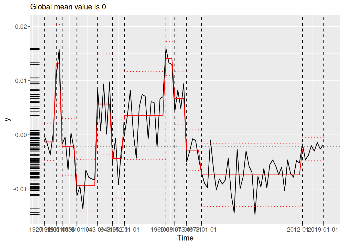
[1] "1929" "1931" "1936" "1943" "1948" "1952" "1966" "1969" "1973" "1978"
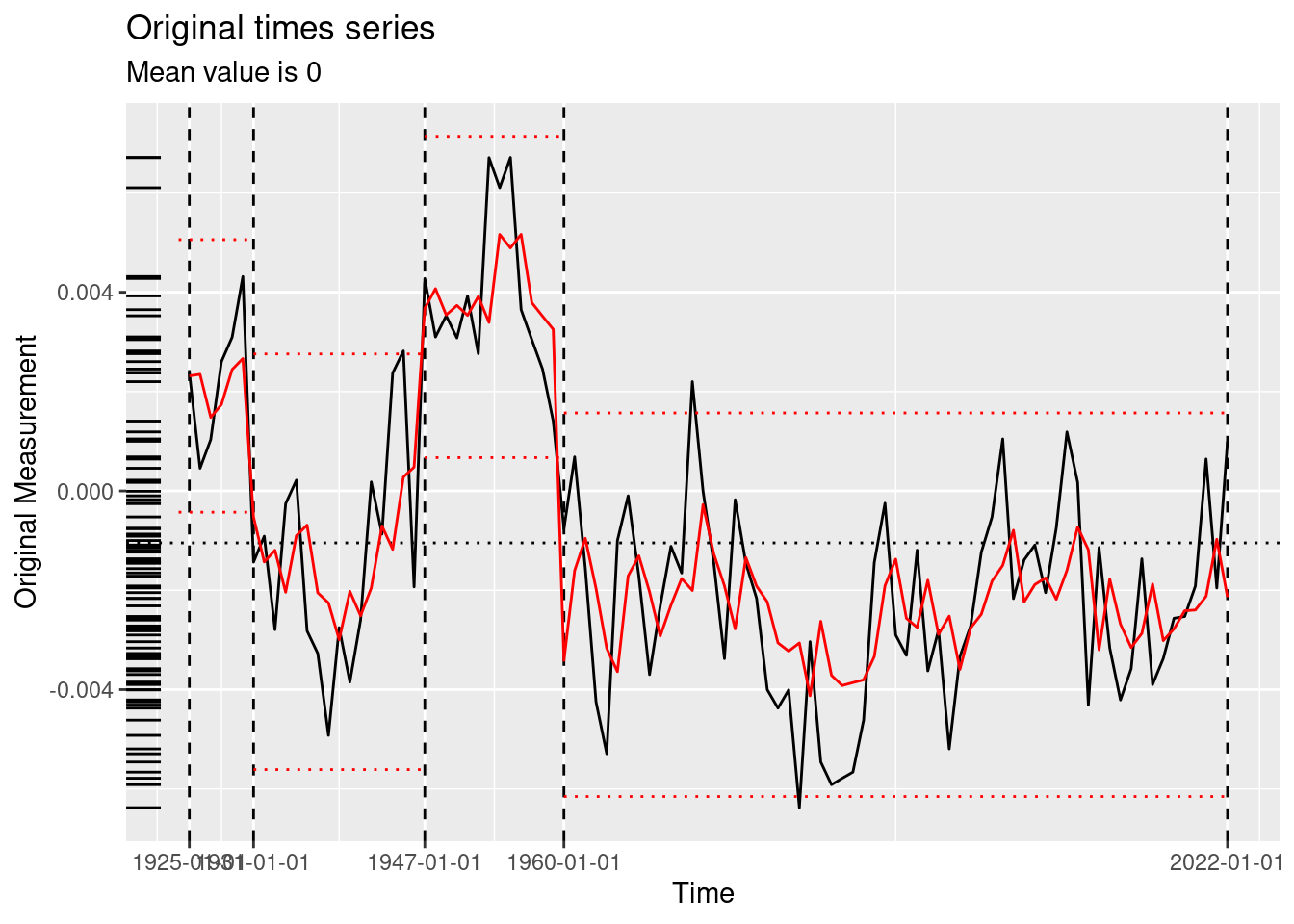
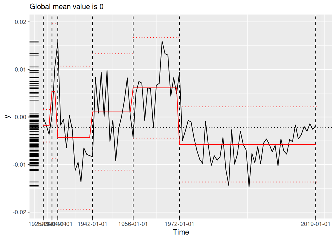
[11] "2012"PELT finds two changepoints, including 1976, which is just three years after the true changepoint of 1973. It also finds 2011 to be a changepoint, which is interesting because the difference in batting average climbs noticeably around this time. PELT using the meanshift model and the BIC penalty finds no changepoints. WBS finds 5 changepoints, including 1972, just one year before the true changepoint. Our genetic algorithm finds 11 changepoints, including the true changepoint.
To compare other aspects of the fits, we can iterate the glance() function from the broom package (Robinson et al. 2026) over that same list. Since glance() always returns a one-row tibble, we can then combine those tibbles into one using the list_rbind() function. Care must be taken to ensure that these comparisons are meaningful. While comparing, say, the elapsed time across these algorithms and models is fair, comparing the fitness values is more fraught. MDL scores are not comparable to BIC or MBIC scores, for example.
In [25]:
mlb_mods |>
  map(glance) |>
  list_rbind()
# A tibble: 4 × 8
pkg version algorithm seg_params model_name criteria fitness elapsed_time
<chr> <pckg_> <chr> <list> <chr> <chr> <dbl> <drtn>
1 changep… 2.3 PELT <list [1]> meanvar MBIC -745. 0.011 secs
2 changep… 2.3 PELT <list [1]> meanshift… BIC -668. 0.002 secs
3 wbs 1.4.1 Wild Bin… <list [1]> meanshift… MBIC -473. 0.010 secs
4 GA 3.2.5 Genetic <list [1]> meanshift… MDL -735. 19.982 secs In Figure 4, we compare the changepoint sets found by the four algorithms. While several of the algorithms indicate a changepoint close to the true changepoint of 1973, it is debatable which provides the best fit to the data.
In [26]:
mlb_mods |>
  map(plot, use_time_index = TRUE)
Scale for x is already present.
Adding another scale for x, which will replace the existing scale.
Scale for x is already present.
Adding another scale for x, which will replace the existing scale.
Scale for x is already present.
Adding another scale for x, which will replace the existing scale.
Scale for x is already present.
Adding another scale for x, which will replace the existing scale.Visually, we could use a rug plot (see ggplot2::geom_rug()) to show the distribution of changepoints across algorithms (see Figure 5). Three of the four algorithms found a changepoint near the true changepoint of 1973. The other changepoints are false positives with respect to the designated hitter rule, but may very well reflect other changes in batting performance that we simply haven’t been thinking about. For example, we hypothesize that the recent decrease in the difference in batting average across the two leagues could be a result of the increased use of relief pitchers (who are almost always replaced by a pinch hitter when their turn at bat comes up) at the expense of starting pitchers (who can’t be pinch-hit for because they have to stay in the game)—a long-term change in pitching strategy. If this trend continued to its extreme and pitchers never batted, the designated hitter rule would be moot and the American League’s advantage would evaporate.
In [27]:
rug <- tibble(
  mod = mlb_mods,
  model = names(mlb_mods)
) |>
  mutate(
    cpts = map(mod, changepoints, use_label = TRUE),
#    cpts = map(cpts, ~c(as.Date("1970-01-01"), .x)),
    mus = map(mod, ~.x$model$region_params$param_mu)
  ) |>
  tidyr::unnest(cpts, keep_empty = TRUE) |>
  mutate(
    bavg_diff = 0,
    yearID = cpts
  )

mlb_plot +
  geom_rug(data = rug, aes(color = model, y = NULL))
Warning: Removed 1 row containing missing values or values outside the scale range
(`geom_rug()`).2.2.1 Investigating algorithmic performance
Because tidychangepoint provides model-fitting functions and penalized objective functions that “just work”, it is easy to investigate why candidate changepoint sets of interest may not have been chosen by the algorithm.
Because PELT is known to be optimal under mild conditions, all other candidate changepoint sets should return a value for MBIC that is worse than the one found by PELT (which includes the two changepoints 1976 and 2011). The fitness() function gives us this value.
In [28]:
fitness(mlb_mods[["pelt_meanvar"]]) MBIC
-744.8353 As expected, the MBIC value of the meanvar model with the true changepoint set is worse (further from \(-\infty\)).
In [29]:
MBIC(fit_meanvar(mlb_bavg, tau = 49))[1] -700.8384Why didn’t PELT pick the changepoint set returned by the genetic algorithm? This set, too, had a worse MBIC score, although its score is better than the true changepoint set.
In [30]:
MBIC(fit_meanvar(mlb_bavg, tau = changepoints(mlb_mods[["ga"]])))[1] -725.6102Alternatively, we might ask why the genetic algorithm didn’t pick either the true changepoint set or the one found by PELT. Recall that the genetic algorithm is randomized and only a heuristic, and so unlike in the case of PELT, it is possible that we could manually identify a changepoint set with a lower MDL than the one found by the algorithm. However, in this case, the MDL score for the changepoint set returned by the genetic algorithms bests the other two possibilities.
In [31]:
fitness(mlb_mods[["ga"]]) MDL
-735.2082 list(49, changepoints(mlb_mods[["pelt_meanvar"]])) |>
map(fit_meanshift_norm, x = mlb_bavg) |>
map_dbl(MDL)[1] -691.7307 -682.8757This type of manual investigation is very difficult to do with other changepoint detection packages.
2.3 Particulate matter in Bogotá, Colombia
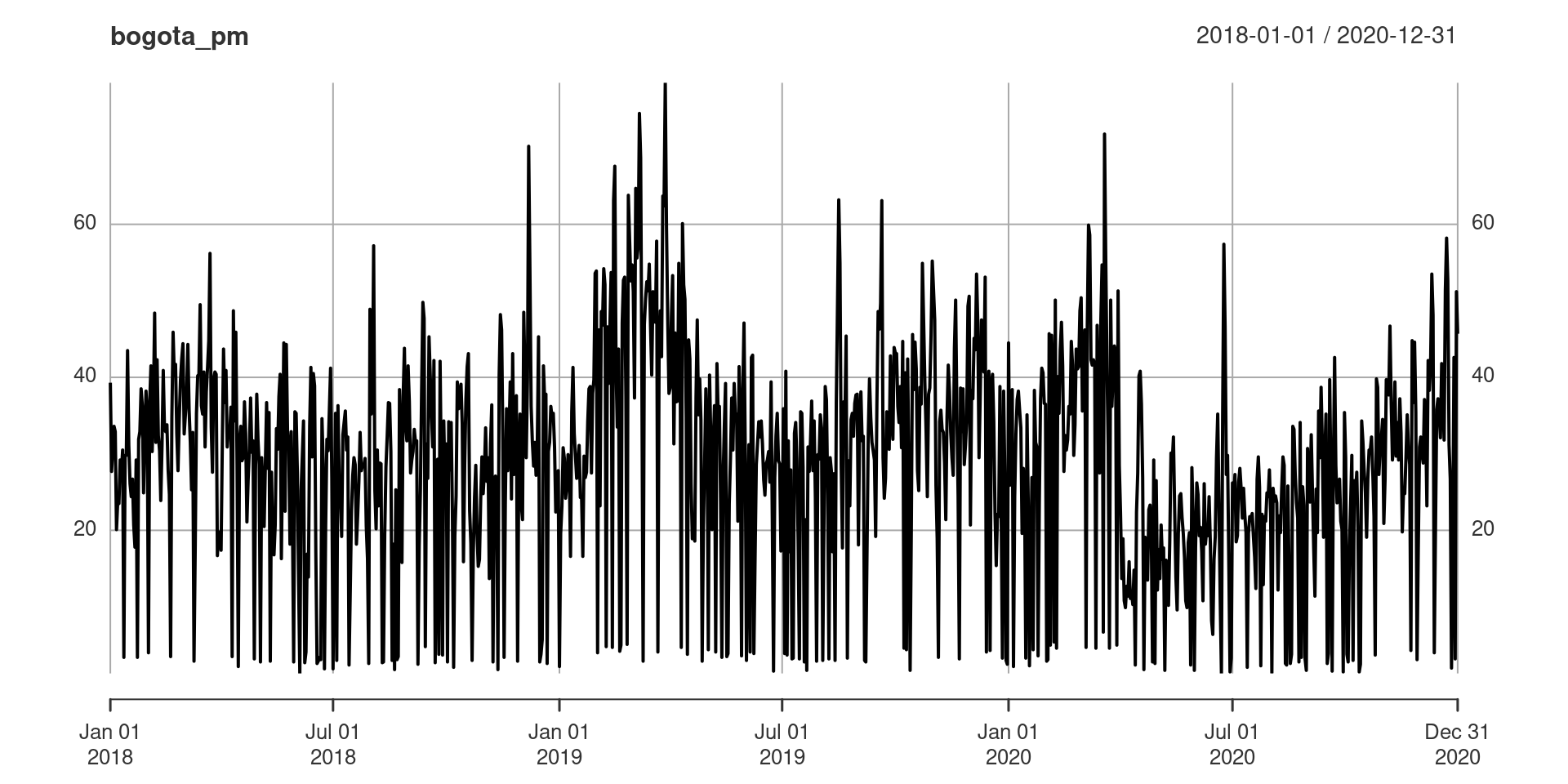
Consider the time series on particulate matter in Bogotá, Colombia collected daily from 2018–2020, discussed in Suárez-Sierra, Coen, and Taimal (2023), and shown in Figure 6. These data are included in tidychangepoint as bogota_pm.
In [32]:
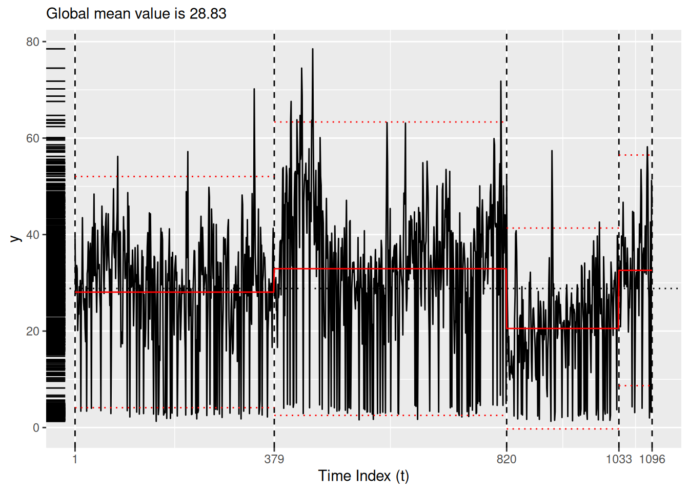
There appears to be some seasonality in the particulate matter data as well as a pronounced drop in particulate matter around the time of the COVID-19 lockdown in March of 2020. Suárez-Sierra, Coen, and Taimal (2023) use Coen’s algorithm (see Section 4.3) with a manually-specified threshold of 37 \(\mu g / m^3\) informed by Colombian government policy. Here, we reproduce that result using the GA-based implementation in tidychangepoint. Although we find a different changepoint set, the fit of the NHPP model is of comparable quality.
In [33]:
bog_coen <- bogota_pm |>
  segment(
    method = "ga-coen", maxiter = 1000, run = 100,
    model_fn_args = list(threshold = 37)
  )
In [34]:
write_rds(bog_coen, file = "bog_coen_500.rds")In [35]:
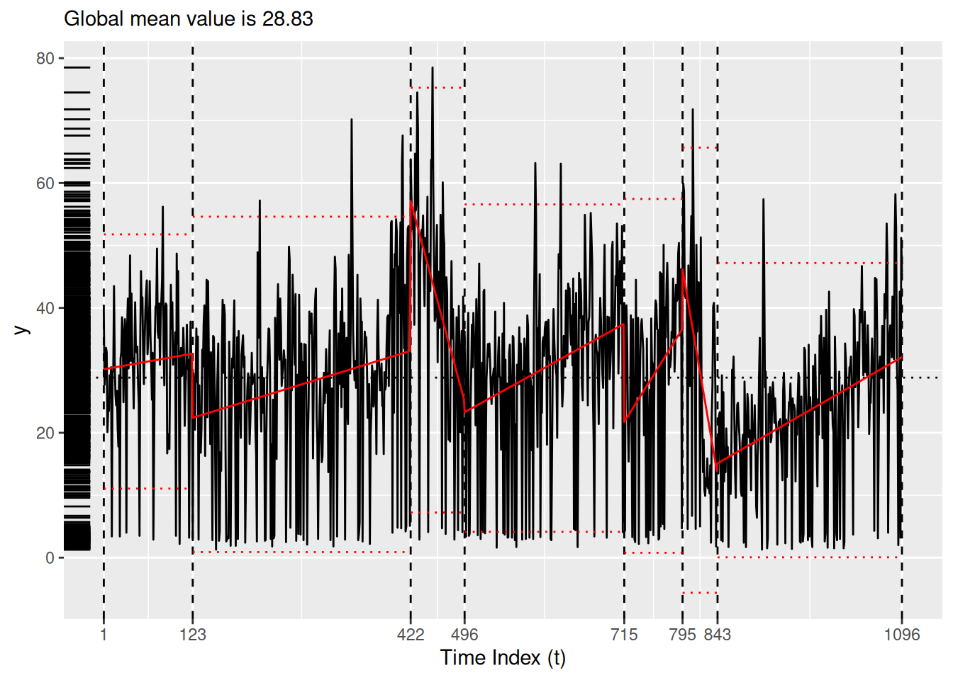
bog_coen <- read_rds("bog_coen_500.rds")A more thorough analysis might use the decompose() or stl() functions from the stats package to unravel the seasonality of the particulate matter data. Instead, for the purposes of simplicity here we simply experiment with different models. Setting the method argument of segment() to ga allows us to employ a custom genetic algorithm for which we can specify a model via the model_fn argument. In this case, we use the fit_lmshift() function (see Section 5.1) to fit a third-degree polynomial (note the model_fn_args argument) to each region. Here, we use the MDL() penalty function and the log_gabin_population() function. Both models in Figure 7 pick up on the COVID-19-related changepoint. The piecewise constant model in Figure 7 (a) ignores the seasonality present in the data, while the Figure 7 (b) is undoubtedly overfit.
In [36]:
bog_ga <- bogota_pm |>
  segment(
    method = "ga", model_fn = fit_trendshift, penalty_fn = MDL,
    population = log_gabin_population(bogota_pm),
    maxiter = 500, run = 100
  )
In [37]:
bog_ga <- bogota_pm |>
  segment(
    method = "ga", model_fn = fit_lmshift,
    model_fn_args = list(deg_poly = 3),
    penalty_fn = MDL,
    population = log_gabin_population(bogota_pm),
    maxiter = 500, run = 100
  )
In [38]:
write_rds(bog_ga, here::here("bogota_pm_ga_500.rda"))In [39]:
bog_ga <- read_rds(here::here("bogota_pm_ga_500.rda"))plot(bog_coen)
plot(bog_ga)Note also that, without running the genetic algorithm again, we can determine that adding AR(1) lagged errors to our model results in an even lower MDL score.
In [40]:
fitness(bog_ga) MDL
8828.881 bogota_pm |>
fit_trendshift_ar1(tau = changepoints(bog_ga)) |>
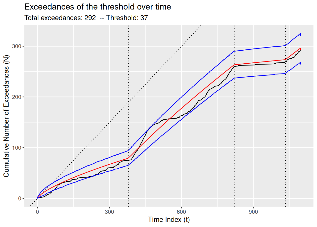
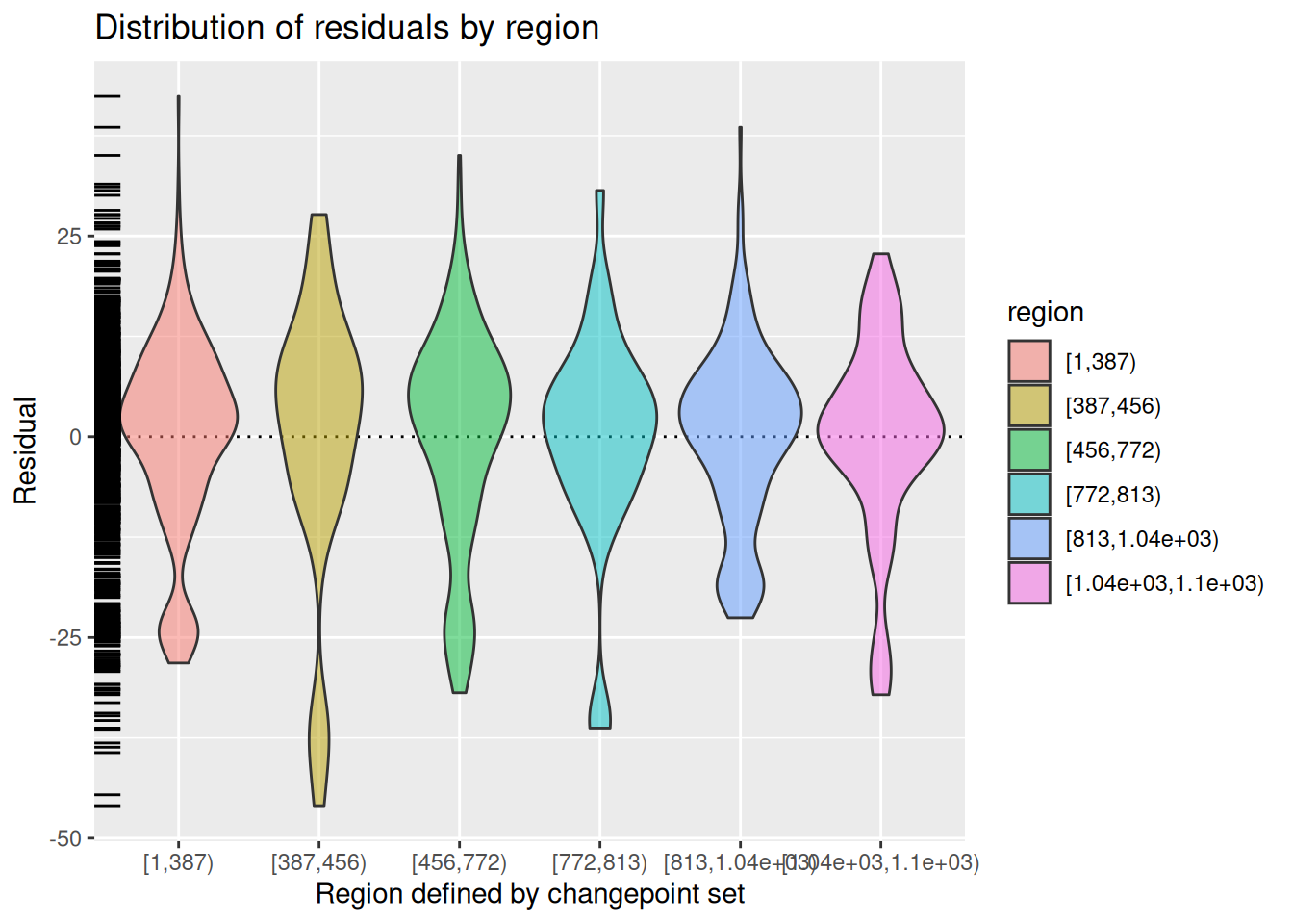
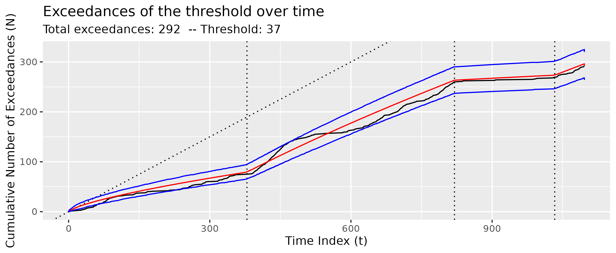
MDL()[1] 8804.22The diagnose() function provides an informative visual understanding of the quality of the fit of the model, which may vary depending on the type of model. In Figure 8, note how Figure 8 (b) summarizes the distribution of the residuals, whereas Figure 8 (a) shows the growth of the cumulative number of exceedances (see Section 5.3) relative to the expected growth based on the NHPP model, with the blue lines showing a 95% confidence interval.
In [41]:
diagnose(as.model(bog_coen))Warning: Removed 1 row containing missing values or values outside the scale range
(`geom_vline()`).ggsave("bog_coen.png", width = 8)Saving 8 x 5 in imageWarning: Removed 1 row containing missing values or values outside the scale range
(`geom_vline()`).ggsave("bog_coen.pdf", width = 8)Saving 8 x 5 in imageWarning: Removed 1 row containing missing values or values outside the scale range
(`geom_vline()`).diagnose(as.model(bog_ga))ggsave("bog_ga.png", width = 8)Saving 8 x 5 in imageggsave("bog_ga.pdf", width = 8)Saving 8 x 5 in imageknitr::include_graphics("bog_coen.png")
knitr::include_graphics("bog_ga.png")3 Architecture of tidychangepoint
The tidychangepoint package implements a simple, flexible structure for working with a myriad of changepoint detection algorithms. tidychangepoint makes extensive use of the S3 object-oriented class system in R. In addition to creating a few new generic functions, it provides methods for a handful of generic functions from other packages (most notably stats and broom) for three new classes of objects (tidycpt, seg_cpt, and mod_cpt), as well as analogous methods for existing objects created by other R packages for changepoint detection (e.g., changepoint). We provide more details in this section.
Every tidycpt object is created by a call to the segment() function. As a verb, “segment” describes the action of splitting a time series into regions, and its usage accords with the tidyverse convention of using verbs as function names. The method argument indicates the algorithm we want to use, and any subsequent arguments (e.g., penalty) are passed to the corresponding function. Here, we pass the penalty argument to force changepoint::cpt.meanvar() to use the BIC penalty function.
In [42]:
mlb_pelt_meanvar_bic <- mlb_bavg |>
  segment(method = "pelt", model_fn = fit_meanvar, penalty = "BIC")
class(mlb_pelt_meanvar_bic)
[1] "tidycpt"3.1 Object structure
Every tidycpt object contains three sub-objects:
segmenter: An object that stores information about an optimal set of changepoints found by an algorithm. Asegmenterobject could be acptobject returned by thecpt.meanvar()function from changepoint, agaobject returned by thega()function from GA, or in principle, any object that provides methods for a few simple generic functions outlined in Section 4.2.model: A model object inheriting frommod_cpt, an internal class for representing model objects. Model objects are created by model-fitting functions, all of whose names start withfit_(see Section 5). Themodelof atidycptobject is the model object returned by thefit_*()function that corresponds to the one used by the segmenter. Because the models described in Section 5 can be fit to any time series based solely on a specified set of changepoints, the information in this object does not depend on the algorithm used to segment the times series: it only depends on the set of changepoints returned by the algorithm.elapsed_time: the clock time that elapsed while the algorithm was running.
3.2 Methods available
tidycpt objects implement methods for the generic functions as.model(), as.segmenter(), as.ts(), changepoints(), diagnose(), fitness(), model_name(), regions(), plot(), and summary(), as well as three generic functions from the broom package: augment(), tidy(), and glance().
In [43]:
methods(class = "tidycpt") [1] as.model as.segmenter as.ts augment changepoints
[6] diagnose fitness glance model_name plot
[11] print regions summary tidy
see '?methods' for accessing help and source codeFor the most part, methods for tidycpt objects typically defer to the methods defined for either the segmenter or the model, depending on the user’s likely intention. To that end, both segmenters and models implement methods for the generic functions as.ts(), changepoints(), model_name(), nobs(), plot(), and print().
In [44]:
intersect(
  methods(class = "mod_cpt") |> attr("info") |> pull("generic"),
  methods(class = "wbs") |> attr("info") |> pull("generic")
)
[1] "as.ts" "changepoints" "model_name" "nobs" "plot"
[6] "print" The changepoints() function returns the time indices of the changepoint set, unless the use_labels argument is set to TRUE.
In [45]:
changepoints(mlb_pelt_meanvar_bic)[1] 15 18 52 87changepoints(mlb_pelt_meanvar_bic, use_labels = TRUE) |>
as_year()[1] "1939" "1942" "1976" "2011"For example, the plot() method for tidycpt simply calls the plot() method for the model of the tidycpt object. The plot shown in Figure 9 uses ggplot2 to illustrate how the proposed changepoint set segments the time series.
In [46]:
Changepoint detection models in tidychangepoint follow the design interface of the broom package. Therefore, augment(), tidy(), and glance() methods exist for mod_cpt objects.
augment()returns atsibble(Wang, Cook, and Hyndman 2020) that is grouped according to the regions defined by the changepoint set. This object class is appropriate for this use case, since the grouping by changepoint region is natural in this context, and atsibbleis a groupedtibblethat is aware of its indexing variable. Users can of course undo the grouping withdplyr::ungroup()or coerce to a regulartibblewithtibble::as_tibble().
In [47]:
augment(mlb_pelt_meanvar_bic)# A tsibble: 95 x 5 [1]
# Groups: region [5]
index y region .fitted .resid
<int> <dbl> <fct> <dbl> <dbl>
1 1 -0.000173 [1,15) -0.00173 0.00156
2 2 -0.00166 [1,15) -0.00173 0.0000703
3 3 -0.00366 [1,15) -0.00173 -0.00192
4 4 0.000285 [1,15) -0.00173 0.00202
5 5 0.0105 [1,15) -0.00173 0.0123
6 6 0.0158 [1,15) -0.00173 0.0175
7 7 -0.00171 [1,15) -0.00173 0.0000243
8 8 -0.000439 [1,15) -0.00173 0.00130
9 9 -0.00650 [1,15) -0.00173 -0.00477
10 10 0.000354 [1,15) -0.00173 0.00209
# ℹ 85 more rowstidy()returns atibble(Müller and Wickham 2026) that provides summary statistics for each region. These include any parameters that were fit, which are prefixed in the output byparam_.
In [48]:
tidy(mlb_pelt_meanvar_bic)# A tibble: 5 × 10
region num_obs min max mean sd begin end param_mu
<chr> <int> <dbl> <dbl> <dbl> <dbl> <dbl> <dbl> <dbl>
1 [1,15) 14 -0.0137 0.0158 -0.00173 0.00779 1 15 -0.00173
2 [15,18) 3 -0.00813 -0.00650 -0.00750 0.000872 15 18 -0.00750
3 [18,52) 34 -0.00923 0.0160 0.00335 0.00628 18 52 0.00335
4 [52,87) 35 -0.0147 -0.000943 -0.00719 0.00315 52 87 -0.00719
5 [87,96) 9 -0.00518 -0.00142 -0.00290 0.00135 87 96 -0.00290
# ℹ 1 more variable: param_sigma_hatsq <dbl>glance()returns a one-rowtibblethat provides summary statistics for the algorithm. This includes the fitness, which is the value of the penalized objective function (see Section 6) that was used.
In [49]:
glance(mlb_pelt_meanvar_bic)# A tibble: 1 × 8
pkg version algorithm seg_params model_name criteria fitness elapsed_time
<chr> <pckg_> <chr> <list> <chr> <chr> <dbl> <drtn>
1 changep… 2.3 PELT <list [1]> meanvar BIC -782. 0.008 secs 4 Segmenters
In the example above, the segmenter is of class cpt, because segment() simply wraps the cpt.meanvar() function from the changepoint package.
In [50]:
mlb_pelt_meanvar_bic |>
  as.segmenter() |>
  class()
[1] "cpt"
attr(,"package")
[1] "changepoint"In addition to the generic functions listed above, segmenters implement methods for the generic functions as.seg_cpt(), fitness(), model_args(), and seg_params().
In [51]:
setdiff(
  methods(class = "wbs") |> attr("info") |> filter(!isS4) |> pull("generic"),
  methods(class = "mod_cpt") |> attr("info") |> pull("generic")
)
[1] "as.seg_cpt" "fitness" "model_args" "seg_params"Note that while tidychangepoint uses only S3 classes, segmenters (such as those of class cpt) may belong to S4 classes. This is one reason why as.seg_cpt(), which coverts a segmenter of any class to a mod_cpt object, is necessary. fitness() returns a named vector with the type and value of the penalized objective function used by the segmenting algorithm.
In [52]:
fitness(mlb_pelt_meanvar_bic) BIC
-782.1165 4.1 Segmenting algorithms provided
Table 1 shows the values passable to the method argument of the segment() function and what they do. Currently, segment() wraps the following algorithms:
- PELT and Binary Segmentation as implemented by changepoint (Killick 2024)
- Wild Binary Segmentation as implemented by wbs (Baranowski and Fryzlewicz 2024)
- Segmented regression models as implemented by strucchange (Zeileis et al. 2024) and segmented (V. M. R. Muggeo 2026)
- A variety of genetic algorithms as implemented by GA (Scrucca 2026) and changepointGA (M. Li and Lu 2025). Specific variants include Shi’s algorithm (Shi et al. 2022) and Coen’s algorithm (Suárez-Sierra, Coen, and Taimal 2023).
- Trivial algorithms for no changepoints, manually input changepoints, and randomly selected changepoints
In [53]:
ls_methods() |>
  arrange(method) |>
  janitor::clean_names(case = "title") |>
  knitr::kable()
In [54]:
| Method | Pkg | Segmenter Class | Helper | Wraps |
|---|---|---|---|---|
| binseg | changepoint | cpt | NA | changepoint::cpt.meanvar() |
| coen | tidychangepoint | seg_basket | segment_coen() | NA |
| cptga | changepointGA | tidycptga | segment_cptga() | changepointGA::cptga() |
| ga | GA | tidyga | segment_ga() | GA::ga() |
| ga-coen | GA | tidyga | segment_ga_coen() | segment_ga() |
| ga-shi | GA | tidyga | segment_ga_shi() | segment_ga() |
| manual | tidychangepoint | seg_cpt | segment_manual() | NA |
| null | tidychangepoint | seg_cpt | segment_manual() | NA |
| pelt | changepoint | cpt | segment_pelt() | changepoint::cpt.mean() or changepoint::cpt.meanvar() |
| random | GA | tidyga | segment_ga_random() | segment_ga() |
| segneigh | changepoint | cpt | NA | changepoint::cpt.meanvar() |
| selgmented | segmented | segmented | NA | segmented::selgmented() |
| single-best | changepoint | cpt | NA | changepoint::cpt.meanvar() |
| stelpmented | segmented | stepmented | NA | segmented::stelpmented() |
| strucchange | strucchange | breakpointsfull | NA | strucchange::breakpoints() |
| wbs | wbs | wbs | NA | wbs::wbs() |
In particular, setting the method argument to the segment() function to ga allows the user to specify any of the model-fitting functions described in Section 5.1 (or a user-defined model-fitting function as in Section 5.2) as well as any of the penalized objective functions in Section 6. While these algorithms can be slow, they are quite flexible.
4.2 Extending tidychangepoint to include new algorithms
In order for a segmenting algorithm to work with tidychangepoint the class of the resulting object must implement, at a minimum, methods for the following generic functions:
- From stats:
as.ts(), andnobs(). These are needed perform basic operations on the time series. - From tidychangepoint:
changepoints()must return a single integer vector with the best changepoint set as defined by the algorithm.fitness()must return a named double vector with the appropriately named value of the penalized objective function.as.segmenter()dumps the contents of the object into amod_cptobject.model_name(),model_args(), andseg_params()provide information about the kind of model that was fit, and any arguments passed to the segmenting function.
These compatibility layers are generally not difficult or time-consuming to write.
4.3 Spotlight: Coen’s algorithm
The goal of Coen’s algorithm (Suárez-Sierra, Coen, and Taimal 2023) is to find the optimal set of changepoints for the NHPP model described in Section 5.3. That is, given a time series \(y\), find the changepoint set \(\tau\) that minimizes the value of \(BMDL(\tau, NHPP(y | \hat{\theta}_\tau))\). To find good candidates, this genetic algorithm starts with a randomly selected set of popSize changepoint sets, and then iteratively “mates” the best (according to the BMDL penalty function, see Section 6.1.4) pairs of these changepoint sets to recover a new “generation” of popSize changepoint sets. This process is repeated until a stopping criteria is met (most simply, maxiter times). Thus, a constant number (popSize \(\times\) maxiter) possible changepoint sets are considered, and the one with the lowest BMDL score is selected.
Coen’s algorithm is implemented in tidychangepoint via the segment() function with the method argument set to ga-coen. As the code below reveals, this is just a special case of the segment_ga() function that wraps GA::ga(). Note that the model_fn argument is set to fit_nhpp and the penalty_fn argument is set to BMDL. The running time of the back-end function GA::ga() is sensitive to the size of the changepoint sets considered, especially in the first generation, and thus we use the population argument to inform the selection of the first generation (see below). Coen’s algorithm runs in about the same time as a naïve algorithm that randomly selects the same number of changepoints, but produces changepoint sets with significantly better BMDL scores.
In [55]:
segment_ga_coenfunction(x, ...) {
segment_ga(
x, model_fn = fit_nhpp, penalty_fn = BMDL,
population = build_gabin_population(x), popSize = 50, ...
)
}
<bytecode: 0x556ab98f6480>
<environment: namespace:tidychangepoint>By default, the function GA::gabin_Population() selects candidate changepoints uniformly at random with probability 0.5, leading to candidate changepoint sets of size \(n/2\), on average. These candidate changepoint sets are usually poor (since \(n/2\) changepoints is ludicrous), and we observe much better and faster performance by seeding the first generation with smaller candidate changepoint sets. To this end, the build_gabin_population() function runs several fast algorithms (i.e., PELT, Wild Binary Segmentation, etc.) and sets the initial probability of being selected to three times the average size of the changepoint set found by these algorithms. This results in much more rapid covergence around the optimal changepoint set. Alternatively, tidychangepoint also provides the log_gabin_population() function, which sets the initial probability to \(\ln{n} / n\) (see Section 7.2).
5 Models
All model objects are created by calls to one of the model-fitting functions listed in Section 5.1, whose name begins with fit_. These functions all inherit from the class fun_cpt and can be listed using ls_models(). All model objects inherit from the mod_cpt base class.
The model object in our example is created by fit_meanvar(), and is of class mod_cpt.
In [56]:
mlb_pelt_meanvar_bic |>
  as.model() |>
  str()
List of 6
$ data : Time-Series [1:95] from 1 to 95: -0.000173 -0.001663 -0.003656 0.000285 0.010521 ...
$ tau : int [1:4] 15 18 52 87
$ region_params: tibble [5 × 3] (S3: tbl_df/tbl/data.frame)
..$ region : chr [1:5] "[1,15)" "[15,18)" "[18,52)" "[52,87)" ...
..$ param_mu : num [1:5] -0.00173 -0.0075 0.00335 -0.00719 -0.0029
..$ param_sigma_hatsq: Named num [1:5] 5.63e-05 5.07e-07 3.83e-05 9.67e-06 1.62e-06
.. ..- attr(*, "names")= chr [1:5] "[1,15)" "[15,18)" "[18,52)" "[52,87)" ...
$ model_params : NULL
$ fitted_values: num [1:95] -0.00173 -0.00173 -0.00173 -0.00173 -0.00173 ...
$ model_name : chr "meanvar"
- attr(*, "class")= chr "mod_cpt"In addition to the generic functions listed above, models implement methods for the generic functions coef(), fitted(), logLik(), plot(), and residuals(), as well as augment(), tidy(), and glance().
In [57]:
setdiff(
  methods(class = "mod_cpt") |> attr("info") |> pull("generic"),
  methods(class = "wbs") |> attr("info") |> filter(!isS4) |> pull("generic")
)
[1] "augment" "coef" "diagnose" "fitted" "glance" "logLik"
[7] "regions" "residuals" "summary" "tidy" Like other model objects that implement glance() methods, the output from the glance() function summarizes the fit of the model to the data.
In [58]:
mlb_pelt_meanvar_bic |>
  as.model() |>
  glance()
# A tibble: 1 × 11
pkg version algorithm params num_cpts rmse logLik AIC BIC MBIC MDL
<chr> <pckg_> <chr> <list> <int> <dbl> <dbl> <dbl> <dbl> <dbl> <dbl>
1 tidy… 1.0.4 meanvar <NULL> 4 0.00507 367. -706. -671. -689. -674.5.1 Model-fitting functions provided
Table 2 lists the model-fitting functions provided by tidychangepoint, along with their parameters. Any of these functions can be passed to the model_fn argument of segment_ga() (see Section 4.1).
In [59]:
tibble::tribble(
  ~`Function name`, ~`$k$`, ~`Parameters ($\\theta$)`, ~Note,
  "`fit_meanshift_norm()`", "$m+2$", "$\\sigma^2, \\mu_0, \\ldots, \\mu_m$", "Normal",
  "`fit_meanshift_lnorm()`", "$m+2$", "$\\sigma^2, \\mu_0, \\ldots, \\mu_m$", "log-normal",
  "`fit_meanshift_pois()`", "$m+2$", "$\\sigma^2, \\mu_0, \\ldots, \\mu_m$", "Poisson",
 "`fit_meanshift_norm_ar1()`", "$m+3$", "$\\sigma^2, \\phi, \\mu_0, \\ldots, \\mu_m$", "",
 "`fit_trendshift()`", "$2m + 3$", "$\\sigma^2, \\mu_0, \\ldots, \\mu_m, \\beta_0, \\ldots, \\beta_m$", "special case of `fit_lmshift()` with $p = 1$",
 "`fit_trendshift_ar1()`", "$2m + 4$", "$\\sigma^2, \\phi, \\mu_0, \\ldots, \\mu_m, \\beta_0, \\ldots, \\beta_m$", "",
 "`fit_lmshift()`", "$p(m + 1) + 1$", "$\\sigma^2, \\beta_{00}, \\ldots, \\beta_{0m}, \\beta_{10}, \\ldots, \\beta_{pm}$", "polynomial[^lm] of degree $p$",
 "`fit_lmshift_ar1()`", "$p(m + 1) + 1$", "$\\sigma^2, \\beta_{00}, \\ldots, \\beta_{0m}, \\beta_{10}, \\ldots, \\beta_{pm}$", "",
 "`fit_meanvar()`", "$2m + 2$", "$\\sigma_0^2, \\ldots, \\sigma_m^2, \\mu_0, \\ldots, \\mu_m$", "",
 "`fit_nhpp()`", "$2m+2$", "$\\alpha_0, \\ldots, \\alpha_m, \\beta_0, \\ldots, \\beta_m$", "",
) |>
  knitr::kable()
In [60]:
_ar1 indicates autocorrelated AR(1) lagged errors (as decribed in Shi et al. (2022)), where \(\phi\) is the measure of autocorrelation. See Section 5.3 for a description of the non-homogeneous Poisson process model used by fit_nhpp().
| Function name | \(k\) | Parameters (\(\theta\)) | Note |
|---|---|---|---|
fit_meanshift_norm() |
\(m+2\) | \(\sigma^2, \mu_0, \ldots, \mu_m\) | Normal |
fit_meanshift_lnorm() |
\(m+2\) | \(\sigma^2, \mu_0, \ldots, \mu_m\) | log-normal |
fit_meanshift_pois() |
\(m+2\) | \(\sigma^2, \mu_0, \ldots, \mu_m\) | Poisson |
fit_meanshift_norm_ar1() |
\(m+3\) | \(\sigma^2, \phi, \mu_0, \ldots, \mu_m\) | |
fit_trendshift() |
\(2m + 3\) | \(\sigma^2, \mu_0, \ldots, \mu_m, \beta_0, \ldots, \beta_m\) | special case of fit_lmshift() with \(p = 1\) |
fit_trendshift_ar1() |
\(2m + 4\) | \(\sigma^2, \phi, \mu_0, \ldots, \mu_m, \beta_0, \ldots, \beta_m\) | |
fit_lmshift() |
\(p(m + 1) + 1\) | \(\sigma^2, \beta_{00}, \ldots, \beta_{0m}, \beta_{10}, \ldots, \beta_{pm}\) | polynomial6 of degree \(p\) |
fit_lmshift_ar1() |
\(p(m + 1) + 1\) | \(\sigma^2, \beta_{00}, \ldots, \beta_{0m}, \beta_{10}, \ldots, \beta_{pm}\) | |
fit_meanvar() |
\(2m + 2\) | \(\sigma_0^2, \ldots, \sigma_m^2, \mu_0, \ldots, \mu_m\) | |
fit_nhpp() |
\(2m+2\) | \(\alpha_0, \ldots, \alpha_m, \beta_0, \ldots, \beta_m\) |
5.2 Extending tidychangepoint to include new models
Users can create their own model-fitting functions. The names of these functions should start with fit_ for consistency, and they must be registered with a call to fun_cpt(). The first argument x must be the time series and the second argument tau must be a subset of the indices of x. Any subsequent arguments can be passed through the dots. Every fit_ function returns an object of class mod_cpt, which can be created with the arguments shown below.
In [61]:
args(new_mod_cpt)function (x = numeric(), tau = integer(), region_params = tibble::tibble(),
model_params = double(), fitted_values = double(), model_name = character(),
...)
NULL5.3 Spotlight: Non-homogenous Poisson process model
Having already described the meanshift model in Section 1, we now describe mathematically the NHPP model used in Coen’s algorithm (see Section 4.3) and created by the fit_nhpp() function listed in Section 5.1.
Let \(z_w(y) = \{t : y_t > w\}\) be a subset of the indices of the original times series \(y\), for which the observation \(y_t\) exceeds some threshold \(w\), which by default is the empirical mean \(\bar{y}\). This new time series \(z_w(y)\) is called the exceedances of the original time series \(y\). Following Suárez-Sierra, Coen, and Taimal (2023), we model the time series \(z_w(y)\) as a non-homogenous Poisson process (NHPP), using a Weibull distribution parameterized by shape (\(\alpha\)) and scale (\(\beta\)). In a Bayesian setting, those parameters follow a Gamma distribution with their appropriate hyperparameters. Thus, we assume that there exists a set of parameters \(\theta = (\alpha_0 \ldots \alpha_m, \beta_0, \ldots, \beta_m)\) for which the exceedances \(z_w(y)\) of the original time series \(y\) are modeled accurately as a non-homogenous Poisson process.
The best-fit parameters are determined by maximizing the log posterior function described below: \[
\ln{ g(\theta_\tau | y ) } \propto \ln{ L_{NHPP}(y | \theta_\tau) } + \ln{ g(\theta_\tau) } \,,
\] where \(L\) is the likelihood function and \(g\) is the prior probability distribution function. Closed-form expressions for each of these components for a Weibull distribution with two Gamma priors are given in Suárez-Sierra, Coen, and Taimal (2023). The tidy() function displays the values of the fitted parameter values, or one can pull the region_params object directly from the model object.
In [62]:
bog_coen |>
  as.model() |>
  pluck("region_params")
# A tibble: 4 × 5
region param_alpha param_beta logPost logLik
<chr> <dbl> <dbl> <dbl> <dbl>
1 [1,379) 0.711 0.808 -202. -198.
2 [379,820) 0.661 0.0762 -346. -344.
3 [820,1.03e+03) 0.484 0.0831 -42.6 -40.6
4 [1.03e+03,1.1e+03) 0.668 0.0788 -48.4 -46.66 Penalized objective functions
We call the function \(f\) a penalized objective function7 because it comes in the form \[
f(\tau, M(y|\theta_\tau)) = \underbrace{P_f(\tau, n)}_{penalty} - 2 \ln{ \underbrace{L_M(y| \theta_\tau)}_{likelihood}} \,,
\] where \(P_f\) is a function that guards against overfitting by penalizing large changepoint sets—that is, it is a monotonically increasing function of \(m\) (the number of changepoints). Recall that \(\tau\) is the set of changepoints. The stats package (R Core Team 2025) provides generic methods for the well-known penalty functions AIC() and BIC(), which work seamlessly on tidychangepoint models because they all implement methods for logLik(). In addition, tidychangepoint provides generic functions and methods for four additional penalty functions: HQC(), MBIC(), MDL(), and BMDL(). For compatibility with changepoint we also provide the alias SIC() for BIC(). tidychangepoint supports all of the penalty functions supported by changepoint, with the exception of the “Asymptotic” and “CROPS” penalties, which are not fully generalizable.
All penalty functions return 0 for the special case in which \(m = 0\). For ease of explanation, let the vector \(\ell_j = \tau_{j+1} - \tau_j\) for \(0 \leq j \leq m\) encode the lengths of the \(m+1\) regions defined by the changepoint set \(\tau\).
6.1 Penalized objective functions supported in tidychangepoint
6.1.1 Hannan-Quinn Information Criterion
The Hannan-Quinn information Criterion is a slight tweak on the BIC that involves an iterated logarithm (Hannan and Quinn 1979): \(P_{HQC}(\tau, n) = 2m \cdot \ln{\ln{n}}\).
6.1.2 Modified Bayesian Information Criterion
Following Zhang and Siegmund (2007) and S. Li and Lund (2012), we define the MBIC as:
\[ P_{MBIC}(\tau, n) = 3 m \ln{n} + \sum_{j=1}^{m+1} \ln{\frac{\ell_j}{n}} \,. \]
6.1.3 Minimum Descriptive Length
As described in Shi et al. (2022) and S. Li and Lund (2012), we define the MDL as:
\[ P_{MDL}(\tau, n) = \frac{a(\theta_\tau)}{2} \cdot \sum_{j=0}^m \log{\ell_j} + 2 \ln{m} + \sum_{j=2}^m \ln{\tau_j} + \left( 2 + b(\theta_\tau) \right) \ln{n} \,, \] where \(a(\theta)\) is the number of parameters in \(\theta\) that are fit in each region, and \(b(\theta)\) is the number of parameters fit to the model as a whole. For example, the in the meanshift model, \(a(\theta) = 1\) to account for the \(\mu_i\)’s, and \(b(\theta) = 1\) to account for \(\sigma^2\).
The MBIC and MDL differ from the penalties imposed by either the Akaike Information Criterion (AIC) or the BIC in important ways. For example, the penalty for the AIC depends just linearly on the number of changepoints, while the BIC depends on the number of changepoints as well as the length of the original times series. Conversely, the MDL penalty depends not only on the number of changepoints, but the values of the changepoints. Because of this, changepoints far from zero can have disproportionate impact.
6.1.4 Bayesian Minimum Descriptive Length
The Bayesian Minimum Descriptive Length combines the MDL penalty function with the log prior \(g\) for the best-fit parameters \(\hat{\theta}\) in the NHPP model described in Section 5.3. Currently, the BMDL penalty can only be applied to the NHPP model.
The exact value of the BMDL is then: \[ BMDL(\tau, NHPP(y | \hat{\theta}_\tau)) = P_{MDL}(\tau) - 2 \ln{ L_{NHPP}(y | \hat{\theta}_\tau) } - 2 \ln{ g(\hat{\theta}_\tau) } \,. \]
6.2 Extending tidychangepoint to include new penalty functions
New penalty functions can be contributed to tidychangepoint by defining a new generic function and implementing a method for the logLik class. Penalty functions should return a double vector of length one.
Note that similar to the logLik() method for lm, the logLik() method for mod_cpt embeds relevant information into the object’s attributes. These include the quantities necessary to compute AIC(), BIC(), MDL(), etc.
In [63]:
mlb_pelt_meanvar_bic |>
  as.model() |>
  logLik() |>
  unclass() |>
  str()
num 367
- attr(*, "num_params_per_region")= int 2
- attr(*, "num_model_params")= int 0
- attr(*, "df")= num 14
- attr(*, "nobs")= int 95
- attr(*, "tau")= int [1:4] 15 18 52 877 Results
In this section we document tidychangepoint’s correctness and computational costs.
7.1 Correctness
Since tidychangepoint relies on other packages to actually segment time series via their respective changepoint detection algorithms, the results returned by segment() are correct to the extent that the dependent results are correct.
However, recall that the model component of a tidycpt object is computed by our fit_*() model-fitting functions, after the segmenting algorithm has returned its results. We show below that these computations are accurate.
First, we match the model parameters returned by fit_trendshift() and fit_trendshift_ar1() with the results for the Central England Temperature data (CET) reported in rows 1–4 of Table 2 in Shi et al. (2022). Unfortunately, the CET data been revised since the publication of Shi et al. (2022), so the temperatures present in CET do not exactly match the temperatures used in Shi et al. (2022) for all years. Accordingly, the numbers in Table 3 do not match exactly, but they are very close. However, when we perform this same analysis on the old data (not shown here), the numbers match exactly.8
In [64]:
cpts <- c(1700, 1739, 1988)
ids <- time2tau(cpts, as_year(time(CET)))
trend_wn <- CET["/2020-01-01"] |>
  fit_trendshift(tau = ids)
trend_ar1 <- CET["/2020-01-01"] |>
  fit_trendshift_ar1(tau = ids)
In [65]:
tibble::tribble(
  ~Model, ~`$\\hat{\\sigma}^2$`, ~logLik, ~BIC, ~MDL, ~`$\\hat{\\phi}$`,
  "@shi2022changepoint WN", 0.291, -290.02, 650.74, 653.07, NA,
  "trend_wn", trend_wn$model_params[["sigma_hatsq"]], as.numeric(logLik(trend_wn)), BIC(trend_wn), MDL(trend_wn), NA,
  "@shi2022changepoint AR(1)", 0.290, -288.80, 654.19, 656.52, 0.058,
  "trend_ar1", trend_ar1$model_params[["sigma_hatsq"]], as.numeric(logLik(trend_ar1)), BIC(trend_ar1), MDL(trend_ar1), trend_ar1$model_params[["phi_hat"]],
) |>
  knitr::kable(digits = c(0, 3, 2, 2, 2, 3))
In [66]:
Second, in Table 4 we compare the estimated parameter values from the model component of a tidycpt object (which are fit by fit_meanvar()) to those from the segmenter component (which are fit by cpt.meanvar()) using a simulated data set.
In [67]:
tidycpt <- DataCPSim |>
  segment(method = "pelt", penalty = "BIC")
# Results shown in Table...
# tidycpt$segmenter@param.est
# y$model$region_params
In [68]:
tidycpt$model$region_params |>
  mutate(
    region = stringr::str_replace(region, "1.1e+0.3", "1096"),
    `$\\hat{\\mu}_{cpt}$` = tidycpt$segmenter@param.est$mean,
    `$\\hat{\\sigma}^2_{cpt}$` = tidycpt$segmenter@param.est$variance,
  ) |>
  rename(
    `$\\hat{\\mu}_{tidycpt}$` = param_mu,
    `$\\hat{\\sigma}^2_{tidycpt}$` = param_sigma_hatsq
  ) |>
  knitr::kable(digits = 2)
# |>
#  kableExtra::add_header_above(header = c(" " = 1, "tidychangepoint" = 2, "changepoint" = 2), escape = FALSE)
In [69]:
fit_meanvar() (\(\hat{\mu}_{tidycpt}\) and \(\hat{\sigma}^2_{tidycpt}\)) to those of changepoint::cpt.meanvar() (\(\hat{\mu}_{cpt}\) and \(\hat{\sigma}^2_{cpt}\)). The discrepancies in the means are caused by tidychangepoint using intervals open on the right, as opposed to the left. Additional discrepancies in the variances are caused by changepoint’s use of the population variance.
| region | \(\hat{\mu}_{tidycpt}\) | \(\hat{\sigma}^2_{tidycpt}\) | \(\hat{\mu}_{cpt}\) | \(\hat{\sigma}^2_{cpt}\) |
|---|---|---|---|---|
| [1,547) | 35.28 | 127.09 | 35.28 | 126.88 |
| [547,822) | 58.10 | 371.75 | 58.20 | 370.52 |
| [822,972) | 96.71 | 923.95 | 96.77 | 920.98 |
| [972,1.1e+03) | 155.85 | 2441.82 | 156.52 | 2405.97 |
The tiny differences in the means are because tidychangepoint uses intervals that are closed on the left and open on the right, whereas changepoint does the opposite. The differences in the variances are caused by the same issue and changepoint’s reporting of the population variance instead of the sample variance.
7.2 Benchmarking
Since segment() wraps underlying functionality from other packages, there is overhead created, both in terms of memory and speed. Table 5 shows the results of benchmarking segment() against changepoint::cpt.meanvar(), which is doing the underlying work in both cases. In this case, segment() uses about twice as much memory and is about 8 times slower than the underlying function. While that may seem like a lot, we’re talking about microseconds.
In [70]:
bench::mark(
  tidychangepoint = segment(mlb_bavg, method = "pelt"),
  changepoint = changepoint::cpt.meanvar(as.ts(mlb_bavg), method = "PELT"),
  check = FALSE,
  iterations = 10
) |>
  select(-result, -memory, -time, -gc) |>
  knitr::kable()
In [71]:
| expression | min | median | itr/sec | mem_alloc | gc/sec | n_itr | n_gc | total_time |
|---|---|---|---|---|---|---|---|---|
| tidychangepoint | 6.13ms | 7.1ms | 134.6282 | 73.2KB | 0 | 10 | 0 | 74.28ms |
| changepoint | 639.47µs | 711.1µs | 1358.2028 | 35.7KB | 0 | 10 | 0 | 7.36ms |
In [72]:
library(tsibble)
aus_retail <- tsibbledata::aus_retail |>
#  tibble::as_tibble() |>
  filter(`Series ID` == "A3349849A") |>
  select(Month, Turnover) |>
  mutate(Month = as_date(Month)) |>
  xts::as.xts()

init_runif <- aus_retail |>
  segment(method = "ga", maxiter = 1000, run = 100)

write_rds(init_runif, file = "init_runif_aus_retail.rds", compress = "xz")

init_build <- aus_retail |>
  segment(
    method = "ga", maxiter = 1000, run = 100,
    population = build_gabin_population(aus_retail)
  )

write_rds(init_build, file = "init_build_aus_retail.rds", compress = "xz")

init_logn <- aus_retail |>
  segment(
    method = "ga", maxiter = 1000, run = 100,
    population = log_gabin_population(aus_retail)
  )

write_rds(init_logn, file = "init_logn_aus_retail.rds", compress = "xz")
In [73]:
init_runif <- read_rds("init_runif_aus_retail.rds")
init_build <- read_rds("init_build_aus_retail.rds")
init_logn <- read_rds("init_logn_aus_retail.rds")
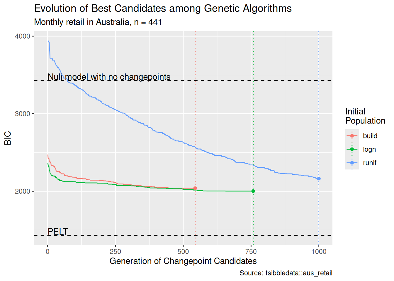
As noted in Section 4.3, tidychangepoint provides two alternative functions to GA::gabin_Population() for creating an initial population for a genetic algorithm: build_gabin_population() and log_gabin_population(). Both perform some näive analysis to set the probability of an observation being selected uniformly at random to belong to the first generation. The former runs three quick algorithms (PELT, Binary Segmentation, and WBS) and sets the probability to three times the average size of the changepoint sets returned by those algorithms, divided by \(n\). The latter sets the probability to \(\log{n}/n\). Both functions can be thought of as “informed” by the data, albeit in different ways. Recall that GA::gabin_Population() always uses the probability \(1/2\), and can thus be considered “uninformed”.
In Figure 10, we compare the performance of a genetic algorithm on monthly retail data from Australia (O’Hara-Wild et al. 2022), using these three methods of forming the initial population. In this test, the maximum number of iterations was set to 1000, with a consecutive run of 100 generations with no improvement stopping the algorithm. We see in Figure 10 that both of the “informed” initial populations result in improved performance. The recovered changepoint sets score better values of the penalized objective function, and both algorithms terminated well before they reached the maximum number of generations. Conversely, the algorithm using the default initial population was still going after 1000 generations. In fact, it only took 35 generations for the BIC scores returned by the genetic algorithm whose initial population was set by log_gabin_population() to beat the best score returned by the same algorithm using the default initial population after 1000 generations.
In [74]:
pdata <- bind_rows(
  init_runif$segmenter@summary |>
    tibble::as_tibble() |>
    dplyr::mutate(
      num_generation = dplyr::row_number(),
      label = "runif"
    ),
  init_build$segmenter@summary |>
    tibble::as_tibble() |>
    dplyr::mutate(
      num_generation = dplyr::row_number(),
      label = "build"
    ),
  init_logn$segmenter@summary |>
    tibble::as_tibble() |>
    dplyr::mutate(
      num_generation = dplyr::row_number(),
      label = "logn"
    )
)

# pdata |>
#   filter(max > -fitness(init_runif)) |>
#   group_by(label) |>
#   slice_head(n = 1)

aus_retail <- init_runif$segmenter@data

benchmarks <- tribble(
  ~num_generation, ~max, ~label,
  0, fitness(segment(aus_retail, method = "null")), "Null model with no changepoints",
  0, fitness(segment(aus_retail, method = "pelt", penalty = "BIC", model_fn = fit_meanshift_norm)), "PELT"
)

endpoints <- tribble(
  ~num_generation, ~max, ~label,
  init_runif$segmenter@iter, -fitness(init_runif), "runif",
  init_build$segmenter@iter, -fitness(init_build), "build",
  init_logn$segmenter@iter, -fitness(init_logn), "logn",
)

ggplot(data = pdata, aes(x = num_generation, y = -max, color = label)) +
  geom_hline(data = benchmarks, aes(yintercept = max), linetype = 2) +
  geom_text(data = benchmarks, aes(label = label, y = max + 50), hjust = "left", color = "black") +
  geom_vline(data = endpoints, aes(xintercept = num_generation, color = label), linetype = 3) +
  geom_line() +
  geom_point(data = endpoints) +
  scale_y_continuous("BIC") +
  scale_x_continuous("Generation of Changepoint Candidates") +
  scale_color_discrete("Initial\nPopulation") +
  labs(
    title = "Evolution of Best Candidates among Genetic Algorithms",
    subtitle = paste("Monthly retail in Australia, n =", length(aus_retail)),
    caption = "Source: tsibbledata::aus_retail"
)Of course, it is possible that by casting a wider net, the default initial population will catch changepoint sets that were randomly excluded by the “informed” initial populations. But these results held up under repeated testing, and they suggest a promising line of attack for future work.
8 Conclusion
8.1 Future work
There is more work to be done to bring additional changepoint detection algorithms, models, and penalty functions into tidychangepoint. Please see the package’s GitHub Issues page for a complete list.
Generally, computational costs for changepoint detection algorithms are a concern. Some algorithms have a known theoretical running time in relation to the length of the time series, while others do not. Moreover, while the implementations of some algorithms (notably, changepoint and GA) use pre-compiled C code, others may not. All of the code for tidychangepoint is written in R, but since it is mainly an interface that wraps code from other packages, the overhead is slight (see Section 7.2), and there isn’t much that can be done to improve performance. Even the new algorithms that are provided by tidychangepoint (e.g., Coen’s algorithm, Shi’s algorithm) are simply special cases of genetic algorithms that use GA as a backend.
Another major issue with changepoint detection algorithms is the robustness of the results to a variety of changes in conditions, assumptions, or computational environments. While some algorithms report the probability of an observation being a changepoint, others do not. Some models rely on assumptions about the distribution or frequency of changepoints relative to the length of the time series. In randomized algorithms (such as genetic algorithms), the robustness of the results may be interrelated with stopping criteria, the initial seed or population, or other computational considerations. CUSUM methods operate on a summary of the original time series: are they less susceptible to outliers? These issues are not correctable within tidychangepoint. We will continue to engage with the authors of the underlying packages when we see areas for improvement and alert our own users to inconsistencies through our documentation.
Finally, in this paper we have considered the multiple changepoint detection problem for a univariate time series, but multivariate time series are also being studied in a variety of contexts.
8.2 Summary
We have described how tidychangepoint offers a flexible but standardized architecture for changepoint detection analysis in R in a manner that is consistent with the design principles of the tidyverse. Previously, changepoint detection analysis could be conducted using a variety of R packages, each of which employed its own non-conforming interface. Our unified interface allows users to compare results across different changepoint algorithms, models, and penalty functions with ease.
References
9 Appendix
changepoint::plot(cet_cpt)
plot(cet_wbs)
plot(cet_bkp)
plot(cet_seg)Note that we have set the maximum number of iterations (generations) to just 1000. To replicate the exact results of Shi et al. (2022) we would need a much larger value. As noted in Section 7.1, the values in the underlying data set have also changed. However, we note that even with different data and many fewer generations, we identified all three of the changepoints found by Shi et al. (2022) to within a year (along with three others).↩︎
Because this analysis leveraged the GA (Scrucca 2026) package, which is not specific to changepoint detection, each model that Shi et al. (2022) wanted to test required writing a different set of code, the complexity of which prevents us from reproducing it here.↩︎
To see why, note that PELT’s reliance on dynamic programming requires that the penalized objective function be additive across the regions. Some penalty functions, such as MDL (see Section 6.1.3) depend on the locations of the changepoints, and thus cannot be additive across the regions.↩︎
purrr::map2()is similar tobase::mapply().↩︎purrr::map()is similar tobase::lapply().↩︎Unlike
fit_meanshift_norm(), thefit_lmshift()function uses thelm()function from the stats, which provides flexibility at the expense of speed (fit_meanshift_norm()is faster).↩︎Occasionally, we may abuse terminology by referring to \(f\) as a penalty function, but technically, \(P_f\) is the penalty function.↩︎
Other results from Table 3 also match.↩︎
