Web scraping and dates
In this lab, we will learn how to use rvest and lubridate to scrape tabular data from web pages, and work with dates and times, respectively.
library(tidyverse)Goal: by the end of this lab, you will be able to pull data from the web directly into R and work sensibly with date/time variables.
Scraping with rvest
The Internet is a great place to get data. We can use rvest to scrape data in HTML tables from the web, but it will often require extensive cleaning before it can be used appropriately.
Consider the following list of largest box office opening weekends:
(http://www.boxofficemojo.com/alltime/weekends/)
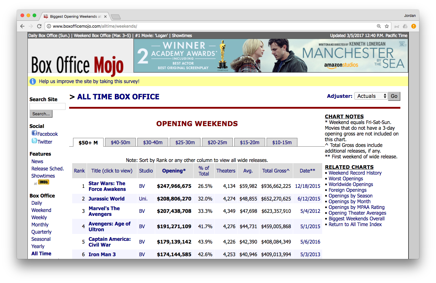
We’ll use rvest to bring this table into R.
library(rvest)
url <- "http://www.boxofficemojo.com/alltime/weekends/"
First, we’ll need to read the contents of the page in HTML. The read_html() function provided by rvest ingests HTML:
html_bom <- read_html(url)
class(html_bom)
html_bom
Unfortunately, this isn’t very readable. What we want is to extract the data that is embedded in the HTML tables. Let’s start by just grabbing those tables, which are inside html table elements. We can use html_nodes() to do this:
tables <- html_bom %>%
  html_nodes("table")
tables
In this case, there is only one table elements on that page (most of them used to create the borders). We are only interested in the big one with all the data. This happens to be the 1st element in the list (note: we figured this out by trial and error).
tables[[1]]The html_table() function will pull the data out of this table and convert it into a data frame. The header = TRUE option tells R that we want to use the first row as our variable names.
movies <- tables[[1]] %>%
  html_table(header = TRUE)
glimpse(movies)
In this case we only had 1 table, so it was not too hard to use trial-and-error to figure out which was the one we wanted. But we could also be a bit more systematic.
Let’s use map() to extract all 6 tables:
list_of_tables <- map(tables, html_table, fill = TRUE)Note that list_of_tables is a list of length 1.
class(list_of_tables)
length(list_of_tables)
str(list_of_tables)
Since html_table() maps HTML tables to data.frames in R, each of the one elements in the list list_of_tables is a data.frame.
map(list_of_tables, class)However, some of the tables are bigger than others.
- Use
map()anddim()to determine the size of each table inlist_of_tables.
map(list_of_tables, dim)It’s obvious from the web page itself that the table we want has 9 variables and 214 rows. Only the 1st element of our list meets that criteria.
Data cleaning
While we now have the data, note that it is very messy:
- the variable names contain special characters, like asterisks, parentheses, and spaces. These can cause problems, so we’ll want to change them.
- most of the columns are stored as
charactervectors, even though they contain quantitative information. In particular, there are columns for dollars, percentages, and dates that are all in the wrong format.
Because of this mismatch, plotting the data will not work as expected.
ggplot(
  data = movies,
  aes(x = Date, y = Opening)
) +
  geom_point(aes(size = `% of Total`))
Note even close to what we want! The parse_number() function from the readr package is extremely useful for cleaning up dollar signs, commas, and percentage signs. We’ll use this in conjunction with the mutate() verb to rename the columns as the same time.
movies <- movies %>%
  mutate(
    opening = parse_number(Opening),
    percent_total = parse_number(`% of Total`)/100
  )
glimpse(movies)
Now when we plot the quantitative data, we get something that makes more sense.
ggplot(data = movies, aes(x = Date, y = opening)) +
geom_point(aes(size = percent_total))- Create a new variable called
num_theatersthat stores the number of theaters as an integer.
movies <- movies %>%
mutate(num_theaters = parse_number(Theaters))- Create new variables for
Avg.andTotal Gross, respectively, that are integers and have names that follow the style guide.
movies <- movies %>%
  mutate(
    avg_gross = parse_number(Average),
    total_gross = parse_number(`Total Gross`)
  )
Dates with lubridate
Unfortunately, the dates are still a problem. Let’s take a closer look at those dates:
movies %>%
  select(Date) %>%
  glimpse()
We see that the dates are in month/day/year format. The lubridate package provides functionality for working with dates, and we can use the mdy() function to convert the character vector into a date class.
library(lubridate)
movies <- movies %>%
  mutate(release_date = mdy(Date))
glimpse(movies)
Now our plot makes sense, especially if we use the scales package to format our axes.
ggplot(data = movies, aes(x = release_date, y = opening)) +
  # We want a scatterplot, and we'll use both color and size to show percent_total
  geom_point(aes(color = percent_total, size = percent_total)) +
  # Clever trick to combine color and size into a single legend
  guides(color = guide_legend("Percent Total"),
         size = guide_legend("Percent Total")) +
  # Format the y-axis to show $ amount
  scale_y_continuous("Opening Day Gross", labels = scales::dollar) +
  # Label our axes
  scale_x_date("Release Date") +
scale_color_viridis_c()- Do the same with this data source: (http://www.the-numbers.com/movie/records/Biggest-Opening-Weekend-at-the-Box-Office)