Mini-Lecture 24

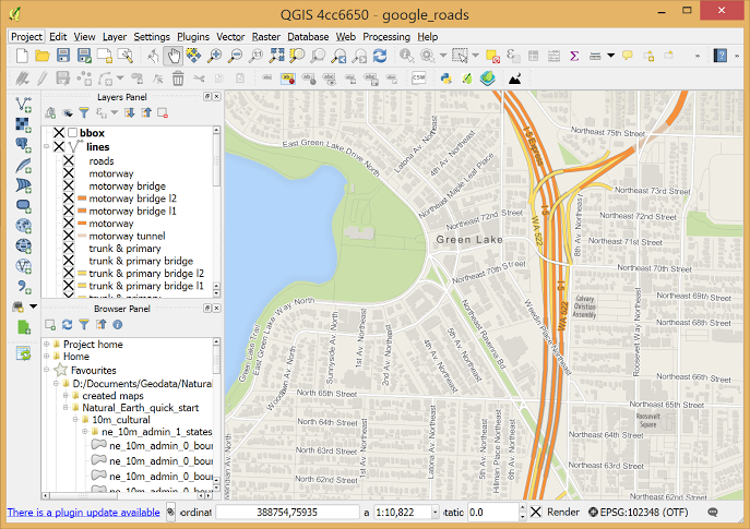
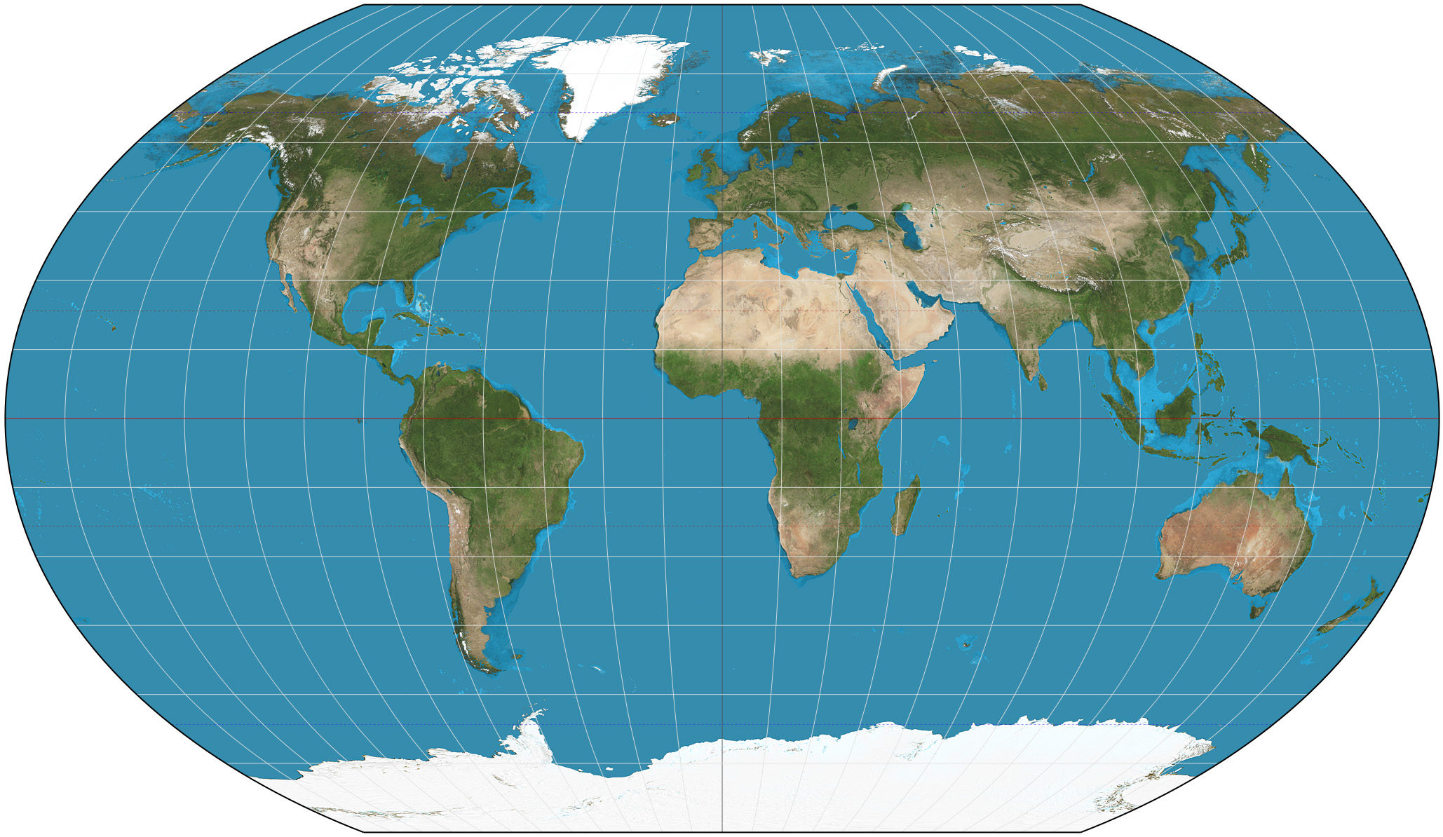
class: center, middle, inverse, title-slide

# Mini-Lecture 24
## Shapefiles and Projections
### Ben Baumer
### SDS 192</br>April 1st, 2019</br>(<a href="http://beanumber.github.io/sds192/lectures/24-shapefiles.html" class="uri">http://beanumber.github.io/sds192/lectures/24-shapefiles.html</a>)

---

class: center, middle
# DataFest recap
---
## `sf`

- Make sure you have `sf` installed

```r
library(sf)
```

```
## Linking to GEOS 3.5.1, GDAL 2.1.3, PROJ 4.9.2
```

- `sf` is installed on `rstudio-dev.smith.edu`
    - same home directory

---
## What to do?

```
package ‘sf’ successfully unpacked and MD5 sums checked

The downloaded binary packages are in
    C:\Users\sgill\AppData\Local\Temp\RtmpC24fvn\downloaded_packages
> devtools::install_github("beanumber/macleish")
Error in loadNamespace(i, c(lib.loc, .libPaths()), versionCheck = vI[[i]]) :
 there is no package called ‘fs’
```

---
## What version of `macleish` do you have?

```
Error in as.double(y) : cannot coerce type ‘S4’ to vector of type ’double.
```

- Need at least version 0.3.3

- Older versions use old `sp` class instead of `sf`

---
## `macleish`

- Make sure you have version >= 0.3.3

- `etl` is a dependency
    - may have to install `RSQLite` package

---
## No vignette?

> Warning message: vignette ‘macleish’ not found" for vignette

- ??

- Not essential -- more of a nice-to-have

---
## `group_map` not found

> It look me a long time and many trials, but I finally was able to download both the macleish and sf packages. The key was that I needed to **update `dplyr`** to version 0.8.0.1.

- `group_map` is a new function!

---
## Joy

.pull-left[

> Btw the interactive maps are suuuuper cool!!! I feel like I'm finally doing what I want to learn :smile:

]

.pull-right[

![](https://media.giphy.com/media/l0ErOU2j8CWarfIAw/giphy.gif)

]

---
## Accessing items in a `data.frame`

```r
names(mtcars)
```

```
##  [1] "mpg"  "cyl"  "disp" "hp"   "drat" "wt"   "qsec" "vs"   "am"   "gear"
## [11] "carb"
```

```r
# vector within a data.frame
mtcars$mpg
```

```
##  [1] 21.0 21.0 22.8 21.4 18.7 18.1 14.3 24.4 22.8 19.2 17.8 16.4 17.3 15.2
## [15] 10.4 10.4 14.7 32.4 30.4 33.9 21.5 15.5 15.2 13.3 19.2 27.3 26.0 30.4
## [29] 15.8 19.7 15.0 21.4
```

```r
# same, tidyverse way
mtcars %>% pull(mpg)
```

```
##  [1] 21.0 21.0 22.8 21.4 18.7 18.1 14.3 24.4 22.8 19.2 17.8 16.4 17.3 15.2
## [15] 10.4 10.4 14.7 32.4 30.4 33.9 21.5 15.5 15.2 13.3 19.2 27.3 26.0 30.4
## [29] 15.8 19.7 15.0 21.4
```

---
## But a `data.frame` is a `list`

```r
class(mtcars)
```

```
## [1] "data.frame"
```

```r
typeof(mtcars)
```

```
## [1] "list"
```

---
# Accessing items in a `data.frame`

```r
class(mtcars["mpg"])
```

```
## [1] "data.frame"
```

```r
class(mtcars[["mpg"]])
```

```
## [1] "numeric"
```

---
## Accessing items in a `list`

```r
library(macleish)
class(macleish_layers)
```

```
## [1] "list"
```

```r
class(macleish_layers["buildings"]) # returns list
```

```
## [1] "list"
```

```r
class(macleish_layers[["buildings"]]) # returns sf
```

```
## [1] "sf"         "data.frame"
```

```r
# tidyverse way
macleish_layers %>%
  pluck("buildings") %>%
  class()
```

```
## [1] "sf"         "data.frame"
```

---
## Selectors

- give me the same kind of thing
    - `[`

- extract the thing and give it to me
    - base R: `$`, `[[`
    - `tidyverse`: `pull()`, `pluck()`

---
## Errors, Warnings, and Messages

.pull-left[

- `error`: code breaks -- you must fix

- `warning`: alert
    - code worked (probably)!
    - read and pay attention
    - often everything is OK

- `message`: just information

]

.pull-right[

![](https://media.giphy.com/media/dtBjNKf61Wqqc/giphy.gif)

]

---
## `leaflet`

> I had trouble adding popups to my interactive map in the last exercise. I **don't fully understand the syntax** for adding layers to the map

> im having trouble **figuring out what the arguments are** for the addPolygon/line to map the data.

- read documentation and examples

- not exactly `ggplot2` syntax

- more practice coming...

---
class: center, middle
# GIS

---
## Geographic Information System (GIS)

.centered[![](http://www.in.gov/gis/images/Capture9.PNG)]

---
## [Smith Spatial Analysis Lab](http://www.science.smith.edu/sal/)

.centered[![](http://www.science.smith.edu/sal/wp-content/uploads/sites/13/2015/03/Banner980x190_1.png)]

- Jon Caris, Director

- Tracy Tien, Spatial Data Specialist

- Smith-specific data

---
## ArcGIS

.centered[![](https://www.arc2earth.com/wp-content/uploads/2014/05/basemaps_sandiego_airports2.png)]

---
## [QGIS](https://www.qgis.org/)

.centered[![](https://www.qgis.org/en/_static/images/about-screenshot.png)]

---
## Spatial packages in R

- Working with shapefiles
    - ~~`sp` for classes and basic functionality~~
    - ~~`rgdal` for projections and advanced reading/writing~~
    - ~~`rgeos` for spatial computations~~
    - `sf` for everything

- Plotting
    - `leaflet` for interactive maps
    - ~~`ggmap` for static maps~~
    - `ggplot2` for static maps

---
## Shapefiles aren't really files

```r
library(sf)
list.files("../../biketrails/")
```

```
## [1] "Bicycle_Trails.lyr"     "biketrails_arc.avl"    
## [3] "biketrails_arc.dbf"     "biketrails_arc.prj"    
## [5] "biketrails_arc.sbn"     "biketrails_arc.sbx"    
## [7] "biketrails_arc.shp"     "biketrails_arc.shp.xml"
## [9] "biketrails_arc.shx"
```

- they all store different information

- but you need *all* of them!

---
## `sf` `data.frame`s

```r
library(macleish)
pluck(macleish_layers, "buildings")
```

```
## Simple feature collection with 27 features and 1 field
## geometry type:  POLYGON
## dimension:      XY
## bbox:           xmin: -72.68251 ymin: 42.44104 xmax: -72.67923 ymax: 42.44919
## epsg (SRID):    4326
## proj4string:    +proj=longlat +datum=WGS84 +no_defs
## First 10 features:
##    name                       geometry
## 1     0 POLYGON ((-72.68056 42.4484...
## 2     0 POLYGON ((-72.68051 42.4483...
## 3     0 POLYGON ((-72.68123 42.4464...
## 4     0 POLYGON ((-72.68116 42.4463...
## 5     0 POLYGON ((-72.68134 42.4461...
## 6     0 POLYGON ((-72.68135 42.4451...
## 7     0 POLYGON ((-72.68137 42.4450...
## 8     0 POLYGON ((-72.68102 42.4445...
## 9     0 POLYGON ((-72.68098 42.4444...
## 10    0 POLYGON ((-72.68143 42.4443...
```

---
## Adding attributes manually

```r
bechtel <- data.frame(lat = 42.449167, lon = -72.679389)
library(leaflet)
leaflet() %>%
  addTiles() %>%
  addMarkers(lng = ~lon, lat = ~lat, data = bechtel,
             popup = "Bechtel Environmental Classroom")
```

<div id="htmlwidget-3f039061120b3500dfbd" style="width:504px;height:360px;" class="leaflet html-widget"></div>
<script type="application/json" data-for="htmlwidget-3f039061120b3500dfbd">{"x":{"options":{"crs":{"crsClass":"L.CRS.EPSG3857","code":null,"proj4def":null,"projectedBounds":null,"options":{}}},"calls":[{"method":"addTiles","args":["//{s}.tile.openstreetmap.org/{z}/{x}/{y}.png",null,null,{"minZoom":0,"maxZoom":18,"tileSize":256,"subdomains":"abc","errorTileUrl":"","tms":false,"noWrap":false,"zoomOffset":0,"zoomReverse":false,"opacity":1,"zIndex":1,"detectRetina":false,"attribution":"© <a href=\"http://openstreetmap.org\">OpenStreetMap<\/a> contributors, <a href=\"http://creativecommons.org/licenses/by-sa/2.0/\">CC-BY-SA<\/a>"}]},{"method":"addMarkers","args":[42.449167,-72.679389,null,null,null,{"interactive":true,"draggable":false,"keyboard":true,"title":"","alt":"","zIndexOffset":0,"opacity":1,"riseOnHover":false,"riseOffset":250},"Bechtel Environmental Classroom",null,null,null,null,{"interactive":false,"permanent":false,"direction":"auto","opacity":1,"offset":[0,0],"textsize":"10px","textOnly":false,"className":"","sticky":true},null]}],"limits":{"lat":[42.449167,42.449167],"lng":[-72.679389,-72.679389]}},"evals":[],"jsHooks":[]}</script>

---
## Adding attributes as variables

```r
bechtel <- data.frame(lat = 42.449167, lon = -72.679389, 
                      name = "Bechtel Environmental Classroom")
leaflet(data = bechtel) %>%
  addTiles() %>%
  addMarkers(lng = ~lon, lat = ~lat, popup = ~name)
```

<div id="htmlwidget-559c1ce18768939593f6" style="width:504px;height:360px;" class="leaflet html-widget"></div>
<script type="application/json" data-for="htmlwidget-559c1ce18768939593f6">{"x":{"options":{"crs":{"crsClass":"L.CRS.EPSG3857","code":null,"proj4def":null,"projectedBounds":null,"options":{}}},"calls":[{"method":"addTiles","args":["//{s}.tile.openstreetmap.org/{z}/{x}/{y}.png",null,null,{"minZoom":0,"maxZoom":18,"tileSize":256,"subdomains":"abc","errorTileUrl":"","tms":false,"noWrap":false,"zoomOffset":0,"zoomReverse":false,"opacity":1,"zIndex":1,"detectRetina":false,"attribution":"© <a href=\"http://openstreetmap.org\">OpenStreetMap<\/a> contributors, <a href=\"http://creativecommons.org/licenses/by-sa/2.0/\">CC-BY-SA<\/a>"}]},{"method":"addMarkers","args":[42.449167,-72.679389,null,null,null,{"interactive":true,"draggable":false,"keyboard":true,"title":"","alt":"","zIndexOffset":0,"opacity":1,"riseOnHover":false,"riseOffset":250},"Bechtel Environmental Classroom",null,null,null,null,{"interactive":false,"permanent":false,"direction":"auto","opacity":1,"offset":[0,0],"textsize":"10px","textOnly":false,"className":"","sticky":true},null]}],"limits":{"lat":[42.449167,42.449167],"lng":[-72.679389,-72.679389]}},"evals":[],"jsHooks":[]}</script>

---
class: center, middle
# Projections

---

background-image: url(https://i.ytimg.com/vi/Lnic0wfHJbE/maxresdefault.jpg)
background-size: contain
---

## Distortion

.centered[![](https://s-media-cache-ak0.pinimg.com/564x/ee/b8/ba/eeb8bafd454afce39587fdb960a55e85.jpg){.cover}]

---
## Projections

- Complicated (non-trivial math)

- There is no one "best" projection

- **Important!!**
    - Not OK to pretend like projections don't matter

- Explore: (https://bl.ocks.org/mbostock/raw/3711652/)

---
## Mercator

![](https://upload.wikimedia.org/wikipedia/commons/f/f4/Mercator_projection_SW.jpg)

---
## [Gall-Peters](https://en.wikipedia.org/wiki/Gall–Peters_projection)

![](https://upload.wikimedia.org/wikipedia/commons/3/34/Gall%E2%80%93Peters_projection_SW.jpg)

---
## Albers Equal Area

![](https://upload.wikimedia.org/wikipedia/commons/4/4f/Kavraiskiy_VII_projection_SW.jpg)

---
## Lambert Conformal Conic

![](https://upload.wikimedia.org/wikipedia/commons/6/67/Lambert_cylindrical_equal-area_projection_SW.jpg)

---
## PROJ.4 strings and EPSG

```r
# GPS and Google Earth
st_crs("+init=epsg:4326")
```

```
## Coordinate Reference System:
##   EPSG: 4326 
##   proj4string: "+proj=longlat +datum=WGS84 +no_defs"
```

```r
# Google Maps*
st_crs("+init=epsg:3857")
```

```
## Coordinate Reference System:
##   EPSG: 3857 
##   proj4string: "+proj=merc +lon_0=0 +lat_ts=0 +x_0=0 +y_0=0 +a=6378137 +b=6378137 +nadgrids=@null +units=m +no_defs"
```

---
## Checking projections

```r
macleish_layers %>%
  pluck("buildings") %>%
  st_crs()
```

```
## Coordinate Reference System:
##   EPSG: 4326 
##   proj4string: "+proj=longlat +datum=WGS84 +no_defs"
```

```r
macleish_layers %>%
  pluck("buildings") %>%
  st_bbox()
```

```
##      xmin      ymin      xmax      ymax 
## -72.68251  42.44104 -72.67923  42.44919
```

---
## Projecting geospatial data

```r
buildings_3857 <- macleish_layers %>%
  pluck("buildings") %>%
  st_transform(3857)

buildings_3857 %>%
  st_crs()
```

```
## Coordinate Reference System:
##   EPSG: 3857 
##   proj4string: "+proj=merc +a=6378137 +b=6378137 +lat_ts=0.0 +lon_0=0.0 +x_0=0.0 +y_0=0 +k=1.0 +units=m +nadgrids=@null +wktext +no_defs"
```

```r
buildings_3857 %>%
  st_bbox()
```

```
##     xmin     ymin     xmax     ymax 
## -8090979  5227276 -8090614  5228505
```

---
## Work on...

- [Lab #15](../lab-sf.html)

- [Homework #5:](../hw/hw_spatial.html)

- [Mini-project #3](../mod_spatial.html)