class: center, middle, inverse, title-slide # Working with Geospatial Data ## sf ### Ben Baumer ### SDS 192</br>April 6th, 2020</br>(<a href="http://beanumber.github.io/sds192/lectures/mdsr_geo_01-sf.html" class="uri">http://beanumber.github.io/sds192/lectures/mdsr_geo_01-sf.html</a>) --- class: center, middle, inverse # `sf` --- ## `sf` is the new hotness .footnote[http://r-spatial.github.io/sf/] .pull-left[ - supersedes older `sp` package - bundles functions from `rgdal` and `rgeos` - spatial objects have class `sf`... - ...but also `data.frame`!! - `tidyverse`-compatible - `dplyr`, `tidyr` verbs - `ggplot2` support ] .pull-right[ .center[] ] <!-- The s f package is the new hotness for geospatial computation in R. It supersedes the older package called s p, and bundles functionality from other geospatial packages like rgeos and rgdal. sf is developed by the same people as those older packages, but it's tidyverse compatible. So, there is no reason to use the older packages. Please be aware of this when you are googling or looking on Stack Overflow. Geospatial objects in sf are data frames! So all of the familiar tools you have to work with data frames, including dplyr and ggplot2, now work with sf objects. --> --- background-image: url(https://user-images.githubusercontent.com/520851/50280460-e35c1880-044c-11e9-9ed7-cc46754e49db.jpg) background-size: contain --- ## How does it work? .footnote[https://github.com/r-spatial/sf] ```r library(sf) ``` ``` ## Linking to GEOS 3.6.2, GDAL 2.2.3, PROJ 4.9.3 ``` -- ```r nc <- system.file("shape/nc.shp", package = "sf") %>% st_read() ``` ``` ## Reading layer `nc' from data source `/home/bbaumer/R/x86_64-pc-linux-gnu-library/3.6/sf/shape/nc.shp' using driver `ESRI Shapefile' ## Simple feature collection with 100 features and 14 fields ## geometry type: MULTIPOLYGON ## dimension: XY ## bbox: xmin: -84.32385 ymin: 33.88199 xmax: -75.45698 ymax: 36.58965 ## CRS: 4267 ``` -- ```r class(nc) ``` ``` ## [1] "sf" "data.frame" ``` --- ## What does it look like? .footnote[https://edzer.github.io/rstudio_conf/#11] ```r nc %>% select(AREA, NAME, geometry) ``` ``` ## Simple feature collection with 100 features and 2 fields ## geometry type: MULTIPOLYGON ## dimension: XY ## bbox: xmin: -84.32385 ymin: 33.88199 xmax: -75.45698 ymax: 36.58965 ## CRS: 4267 ## First 10 features: ## AREA NAME geometry ## 1 0.114 Ashe MULTIPOLYGON (((-81.47276 3... ## 2 0.061 Alleghany MULTIPOLYGON (((-81.23989 3... ## 3 0.143 Surry MULTIPOLYGON (((-80.45634 3... ## 4 0.070 Currituck MULTIPOLYGON (((-76.00897 3... ## 5 0.153 Northampton MULTIPOLYGON (((-77.21767 3... ## 6 0.097 Hertford MULTIPOLYGON (((-76.74506 3... ## 7 0.062 Camden MULTIPOLYGON (((-76.00897 3... ## 8 0.091 Gates MULTIPOLYGON (((-76.56251 3... ## 9 0.118 Warren MULTIPOLYGON (((-78.30876 3... ## 10 0.124 Stokes MULTIPOLYGON (((-80.02567 3... ``` --- ## Every `sf` object has a `geometry` ```r nc %>% st_geometry() %>% pluck(1) ``` ``` ## MULTIPOLYGON (((-81.47276 36.23436, -81.54084 36.27251, -81.56198 36.27359, -81.63306 36.34069, -81.74107 36.39178, -81.69828 36.47178, -81.7028 36.51934, -81.67 36.58965, -81.3453 36.57286, -81.34754 36.53791, -81.32478 36.51368, -81.31332 36.4807, -81.26624 36.43721, -81.26284 36.40504, -81.24069 36.37942, -81.23989 36.36536, -81.26424 36.35241, -81.32899 36.3635, -81.36137 36.35316, -81.36569 36.33905, -81.35413 36.29972, -81.36745 36.2787, -81.40639 36.28505, -81.41233 36.26729, -81.43104 36.26072, -81.45289 36.23959, -81.47276 36.23436))) ``` --- ## Can we see it? ```r nc %>% select("AREA", geometry) %>% * plot() ``` 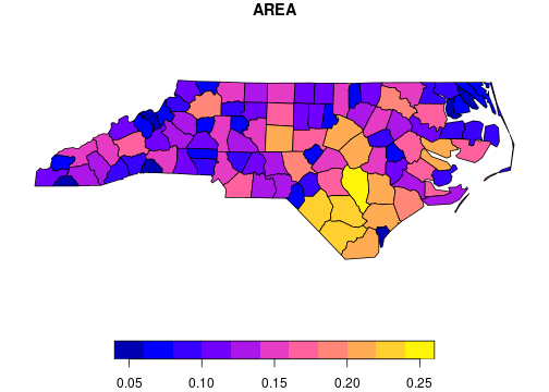<!-- --> --- ## `ggplot2` support - Use `geom_sf()` - mapping `(x, y)` to `geometry` is **implied!** ```r ggplot(nc, aes(fill = AREA)) + geom_sf() ``` 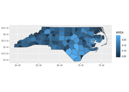<!-- -->