07: Linear fit

IMS, Ch. 7

Benjamin S. Baumer

Smith College

Feb 11, 2026

Warmup

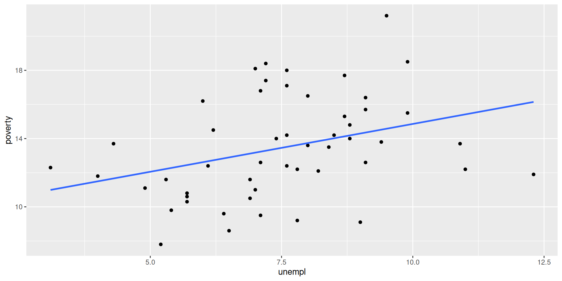
Poverty and Unemployment

Research Question

• Is there an association between poverty and unemployment among states? (among all 50 states and the District of Columbia, as of 2020)

library(tidyverse)
library(usdata)
ggplot(state_stats, aes(x = unempl, y = poverty)) + 
  geom_point() +
  geom_smooth(method = "lm", se = 0)

Your turn: SLR by hand!

Problem

• Use summary statistics to calculate the OLS regression line by hand!

state_stats |>
  summarize(
    num_obs = n(),
    mean_poverty = mean(poverty), 
    sd_poverty = sd(poverty),
    mean_unempl = mean(unempl),
    sd_unempl = sd(unempl),
    correl = cor(poverty, unempl)
  )

# A tibble: 1 × 6
  num_obs mean_poverty sd_poverty mean_unempl sd_unempl correl
    <int>        <dbl>      <dbl>       <dbl>     <dbl>  <dbl>
1      51         13.5       3.02        7.50      1.83  0.340

• Recall that \((\bar{x}, \bar{y})\) is always on the OLS line!

Your turn: Interpretations

• Value of slope (\(b_1\)):
• Value of intercept (\(b_0\)):
• Write an interpretation of:
  • slope:
  • intercept:

A residual

state_stats |>
  filter(state == "Massachusetts") |>
  select(state, abbr, poverty, unempl)

# A tibble: 1 × 4
  state         abbr  poverty unempl
  <fct>         <fct>   <dbl>  <dbl>
1 Massachusetts MA       10.5    6.9

• What is the expected poverty rate for Massachusetts (\(\hat{y}_{MA}\))?
• What is the residual for Massachusetts (\(e_{MA}\))?

Measuring the Strength of Fit

\(R^2\)

• percentage of variation in the response variable (\(y\)) that is explained by the explanatory variables.
• coefficient of determination
• \(R^2\) is always between 0 and 1
• For simple linear regression only (one explanatory variable), \(R^2 = r^2\)
• \(R^2 = 1 - SSE/SST = SSM/SST\)
• Recall this picture

\(SST\), in R

• Sum of squares (\(SST\)) has only to do with the response

response_summary <- state_stats |>
  summarize(
    n = n(),
    SST = sum((poverty - mean(poverty))^2),
    # alternative formulation using sample variance
    SST_alt = var(poverty) * (n - 1)
  )
response_summary

# A tibble: 1 × 3
      n   SST SST_alt
  <int> <dbl>   <dbl>
1    51  457.    457.

• Sum of squares of the null model
• Null model has \(R^2\) of 0 (Why?)

\(SSE\), in R

• \(SSE\) has to do with the model

mod <- lm(poverty ~ unempl, data = state_stats)

• Use the broom package to work with model objects

library(broom)
model_summary <- mod |>
  augment() |>
  summarize(
    n = n(),
    SSE = sum(.resid^2),
    # alternative formulation using sample variance
    SSE_alt = var(.resid) * (n - 1)
  )
model_summary

# A tibble: 1 × 3
      n   SSE SSE_alt
  <int> <dbl>   <dbl>
1    51  404.    404.

\(R^2\), in R

# compute directly, just for today!
1 - model_summary$SSE / response_summary$SST

[1] 0.115497

# using broom::glance()
glance(mod)

# A tibble: 1 × 12
  r.squared adj.r.squared sigma statistic p.value    df logLik   AIC   BIC
      <dbl>         <dbl> <dbl>     <dbl>   <dbl> <dbl>  <dbl> <dbl> <dbl>
1     0.115        0.0974  2.87      6.40  0.0147     1  -125.  256.  262.
# ℹ 3 more variables: deviance <dbl>, df.residual <int>, nobs <int>

# using summary()
summary(mod)

Call:
lm(formula = poverty ~ unempl, data = state_stats)

Residuals:
    Min      1Q  Median      3Q     Max 
-5.1974 -1.8006 -0.2719  1.9045  6.6224 

Coefficients:
            Estimate Std. Error t value Pr(>|t|)    
(Intercept)   9.2528     1.7107   5.409 1.88e-06 ***
unempl        0.5605     0.2216   2.529   0.0147 *  
---
Signif. codes:  0 '***' 0.001 '**' 0.01 '*' 0.05 '.' 0.1 ' ' 1

Residual standard error: 2.873 on 49 degrees of freedom
Multiple R-squared:  0.1155,    Adjusted R-squared:  0.09745 
F-statistic: 6.398 on 1 and 49 DF,  p-value: 0.01469

RailTrail

• Recall the RailTrail example
• Consider two models (shown here):
  • a null model in based strictly on the average volume (left)
  • a linear regression model for \(volume\) as a function of \(avgtemp\) (right).

Your turn: RailTrail

• Use glance() to compute the \(R^2\) value for the second model:
• What is the \(R^2\) for the first model?
• Which one fit the data better?
• Write a sentence interpreting the \(R^2\) for the second model