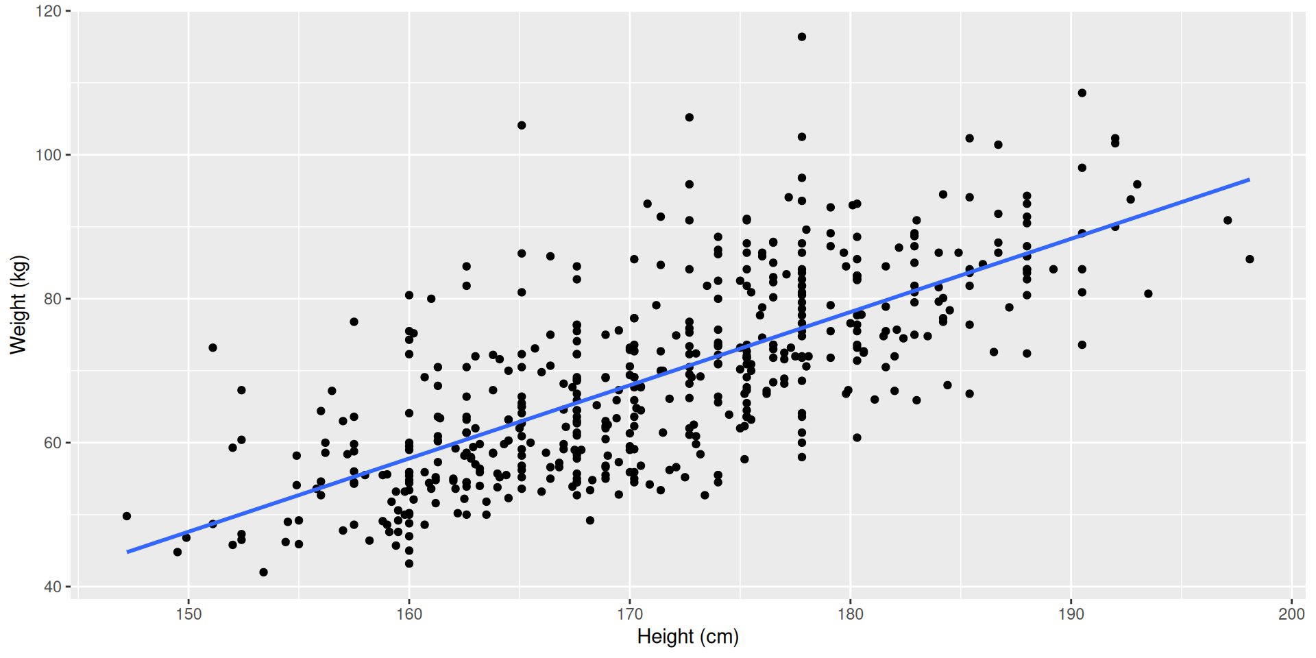
08: Outliers and Leverage

IMS, Ch. 7

Smith College

Feb 13, 2026

Recap

Sums of squares decomposition

\[ y_i - \bar{y} = y_i + (\hat{y}_i - \hat{y}_i) - \bar{y} \]

Rearrange terms:

\[ \underbrace{y_i - \bar{y}}_{\text{null residual}} = (\underbrace{y_i - \hat{y}_i}_{\text{model residual}}) + (\underbrace{\hat{y}_i - \bar{y}}_{\text{model improvement}}) \]

It can be shown that (not obvious):

\[ \underbrace{\sum_{i} (y_i - \bar{y})^2}_{SST} = \underbrace{\sum_{i} (y_i - \hat{y}_i)^2}_{SSE} + \underbrace{\sum_{i} (\hat{y}_i - \bar{y})^2}_{SSM} \]

Warmup

Body dimensions

Consider the relationship between weight (kilograms) and height (centimeters) of 507 physically active individuals.

library(tidyverse)
library(openintro)
data_space <- ggplot(bdims, aes(x = hgt, y = wgt)) +
  geom_point() + 
  geom_smooth(method = "lm", se = 0) + 
  scale_x_continuous("Height (cm)") + 
  scale_y_continuous("Weight (kg)")

Body dimensions

data_space
lm(wgt ~ hgt, data = bdims) |>
  coef()
(Intercept)         hgt 
-105.011254    1.017617 

Your turn: Body dimensions

  • Describe the relationship between height and weight.
  • Write the equation of the regression line
  • Interpret the slope and intercept in context
  • The correlation coefficient for height and weight is 0.72. Calculate \(R^2\) and interpret it in context.

Outliers, Leverage, and Influence

Outliers

  • outlier: an observation that doesn’t seem to fit the general pattern of the data
  • An observation with an extreme value of the explanatory variable is a point of high leverage
  • A high leverage point that exerts disproportionate influence on the slope of the regression line is an influential point
  • important to identify
  • must understand role in determining the regression line
  • don’t just throw them out without a good reason!

True or False?

  • High leverage points always change the intercept of the regression line
  • High leverage points are always close to \(\bar{x}\)
  • It is much more likely for a low leverage point to be influential, than a high leverage point

Regression with categorical variable

One Categorical Explanatory Variable

Recall the RailTrail example

  • \(weekday\) is binary and takes on the values 0 and 1
  • [Such variables are often called indicator variables (by mathematicians) or dummy variables (by economists).]
  • A model using weekday has the form:

\[ \widehat{volume} = \hat{\beta}_0 + \hat{\beta}_1 \cdot weekday \]

RailTrail with weekday

library(mosaic)
ggplot(RailTrail, aes(y = volume, x = weekday)) + 
  geom_jitter(width = 0.05, height = 0)
lm(volume ~ weekday, data = RailTrail) |>
  coef()
(Intercept) weekdayTRUE 
  430.71429   -80.29493 

Your turn: RailTrail predictions

  • How many riders does the model expect will visit the RailTrail on a weekday?
  • What about a weekend?
  • What if it’s 80 degrees out?
  • How would you draw this model on the scatterplot?
  • Estimate the \(R^2\) for this model. Is it greater or less than the \(R^2\) for the model with temperature as an explanatory variable?