09: Parallel Slopes

IMS, Ch. 8

Smith College

Feb 16, 2026

Multiple Regression

SLR: in brief

  • SLR: one response variable, one explanatory variable \[ y = \beta_0 + \beta_1 \cdot X + \epsilon \]

MLR: in brief

  • a natural extension of simple linear regression
  • one response variable, more than one explanatory variable \[ y = \beta_0 + \beta_1 \cdot X_1 + \beta_2 \cdot X_2 + \cdots + \beta_p \cdot X_p + \epsilon \]
  • Estimated coefficients (\(\hat{\beta}_i\)’s) now interpreted in relation to (or “conditional on”) the other variables
  • \(\beta_i\) reflects the change in \(y\) associated with a one unit increase in \(X_i\), conditional upon the rest of the \(X_i\)’s.
  • \(R^2\) has the same interpretation (proportion of variability explained by the model)

Parallel slopes

MLR: Parallel slopes

Consider the case where \(X_1\) is numerical, but \(X_2\) is an indicator variable that can only be 0 or 1 (e.g., \(isCat\)). \[ \widehat{weight} = b_0 + b_1 \cdot height + b_2 \cdot isCat \]

So then, \[\begin{align*} \text{For dogs, } \qquad \widehat{weight} |_{ X_1, X_2 = 0} &= b_0 + b_1 \cdot height \\ \text{For cats, } \qquad \widehat{weight} |_{ X_1, X_2 = 1} &= b_0 + b_1 \cdot height + b_2 \cdot 1 \\ &= \left( b_0 + b_2 \right) + b_1 \cdot X_1 \end{align*}\]

  • This is called a parallel slopes model. [Why?]

Example: Italian Restaurants

  • Want to understand variation in average \(Price\) of a dinner for two in Italian restaurants in New York City.
  • Customer ratings (measured on a scale of 0 to 30) of the \(Food\), \(Decor\), and \(Service\)
  • Located to the \(East\) or west of 5th Avenue
  • 168 Italian restaurants in 2001

Italian restaurants data

library(tidyverse)
nyc <- read_csv("https://gattonweb.uky.edu/faculty/sheather/book/docs/datasets/nyc.csv")
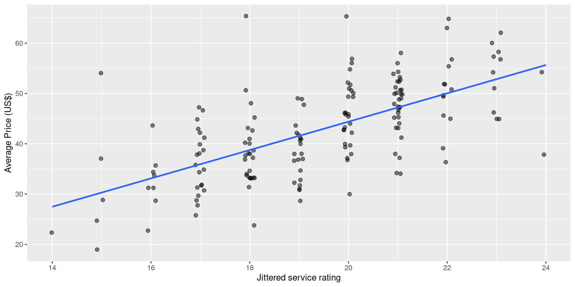
ggplot(data = nyc, aes(x = Service, y = Price)) +
  geom_jitter(width = 0.1, alpha = 0.5, size = 2) + 
  geom_smooth(method = "lm", se = 0) +
  xlab("Jittered service rating") + 
  ylab("Average Price (US$)")

Model in terms of \(Service\)

lm(Price ~ Service, data = nyc)

Call:
lm(formula = Price ~ Service, data = nyc)

Coefficients:
(Intercept)      Service  
    -11.978        2.818  

Interpretation of Slope

  • Among Italian restaurants in NYC in 2001, each additional rating point of service is associated with a $2.82 increase the expected price of a meal for two.

Your turn: Exploratory data analysis

  • Use ggplot() to examine the bivariate relationships between \(Price\), \(Food\) and \(Service\)
  • What do you observe? Describe the form, direction, and strength of the relationships

Your turn: SLR for \(Food\)

  • Use lm() to build a SLR model for \(Price\) as a function of \(Food\)
  • Interpret the coefficients of this model
  • How is the quality of the food at these restaurants associated with its price?

Your turn: Parallel slopes model

  • Build a parallel slopes model by conditioning on the \(East\) variable
  • Interpret the coefficients of this model
  • What is the value of being on the East Side of Fifth Avenue?