library(tidyverse)
nyc <- read_csv("https://gattonweb.uky.edu/faculty/sheather/book/docs/datasets/nyc.csv")
mod <- lm(Price ~ Food + East, data = nyc)
italian_plot <- ggplot(
data = nyc,
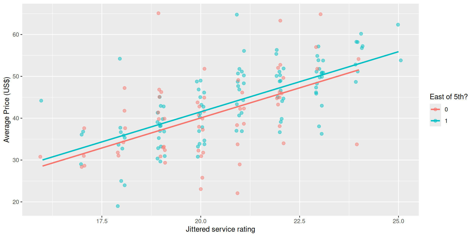
aes(x = Food, y = Price, color = factor(East))
) +
geom_jitter(width = 0.1, alpha = 0.5, size = 2) +
scale_x_continuous("Jittered service rating") +
scale_y_continuous("Average Price (US$)") +
scale_color_discrete("East of 5th?")10: Multiple Linear Regression
IMS, Ch. 8
Smith College
Feb 18, 2026
Recap
Recall the Italian restaurants data
Parallel slopes model
Model interpretation
Interpretation of Slope
- Among Italian restaurants in NYC in 2001, each additional rating point of Food is associated with a $2.88 increase the expected price of a meal of two, after controlling for location (relative to 5th Avenue).
Interpretation of East
- On average, restaurants on the East side of 5th Avenue charge $1.46 more (than those on the West side) for food of the same quality.
Your turn: Parallel slopes model
How is the quality of the \(Decor\) at these restaurants associated with its price?
Build a parallel slopes model by conditioning on the \(East\) variable. Interpret the coefficients of this model.
What is the value of being on the East Side of Fifth Avenue?
Calculate the expected \(Price\) of a restaurant in the East Village with a \(Decor\) rating of 23.
Multiple Regression with a Second Quantitative Variable
MLR: two numerical explanatory variables
If \(X_2\) is a quantitative variable, then we have
\[ \widehat{y} = b_0 + b_1 \cdot X_1 + b_2 \cdot X_2 \]
Notice that our model is no longer a line, rather it is a plane that lives in three dimensions!
Italian Restaurants (continued)
- Consider quality of \(Food\), and also quality of \(Service\)
- In R, simply add another variable to our model
Your turn
Interpret the value of the \(Food\) coefficient
Interpret the value of the \(Service\) coefficient
3D plotting with plotly
- Set up a grid of values in the
Food-Serviceplane
Build the 3D plot
3D visualization
Your turn: interpretation
- Interpret the coefficients of this model:
- What does the coefficient of \(Food\) mean?
- \(Service\)?
- How important is \(Service\) relative to \(Food\)?
- Is it fair to compare the two coefficients?
Your turn: residuals
- Use
broom::augment()to find the expected \(Price\) of a restaurant with a \(Food\) rating of 21 and a \(Service\) rating of 28 - Calculate the residual for San Pietro. Is it overpriced?
Higher dimensions
- What geometric shape would we have if we added all three explanatory variables to the model?
mod_full <- lm(Price ~ Food + Service + East, data = nyc)

planes <- nyc |>
  data_grid(
    Food = seq_range(Food, n = 25),
    Service = seq_range(Service, n = 25),
    East = seq_range(East, n = 2)
  )

planes <- planes |>
  mutate(Price_hat = predict(mod_full, newdata = planes))

pplanes <- data_space_fs |>
  add_surface(
    data = filter(planes, East == 0),
    x = ~unique(Food), y = ~unique(Service),
    z = ~matrix(Price_hat, nrow = 25),
    opacity = 0.7
  ) |>
  add_surface(
    data = filter(planes, East == 1),
    x = ~unique(Food), y = ~unique(Service),
    z = ~matrix(Price_hat, nrow = 25),
    opacity = 0.7
  )
Big reveal
![]()