# A tibble: 35 × 6
       X     Y     Z     W color    id
   <dbl> <dbl> <dbl> <dbl> <chr> <int>
 1   6     6      10    10 black     1
 2   6     6      10    10 black     2
 3   5.7   6       9     9 black     3
 4   3.6   3.5     4     1 white     4
 5   5.1   6       9     7 black     5
 6   5.9   6       9     9 black     6
 7   5.7   6       9     9 black     7
 8   6     6      10    10 black     8
 9   5.6   6      10     9 black     9
10   3.2   4       5     2 white    10
# ℹ 25 more rowsSampling Distributions
IMS, Ch. 12
Mar 6, 2026
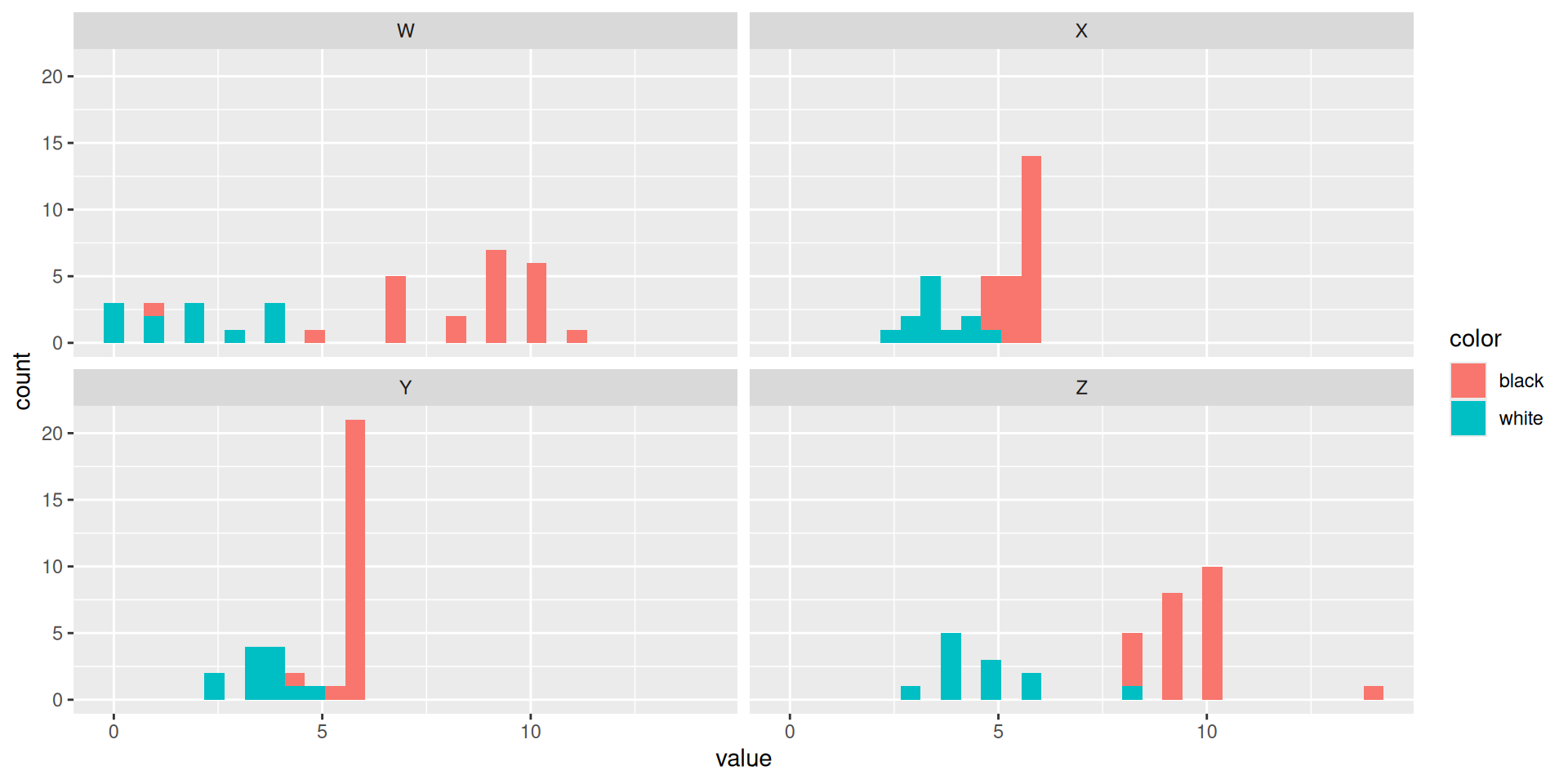
View distribution of r.v.’s
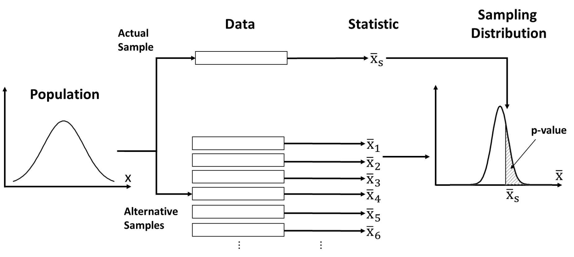
Sampling distribution


What if we resample from our sample?
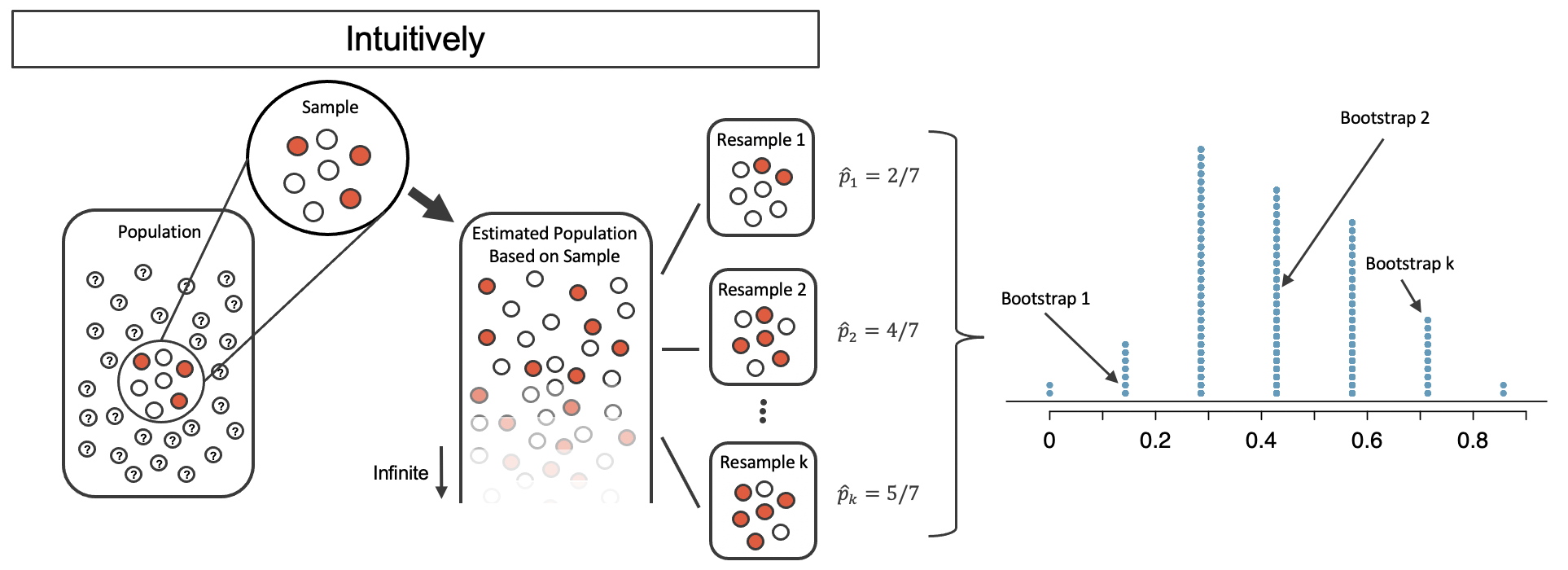
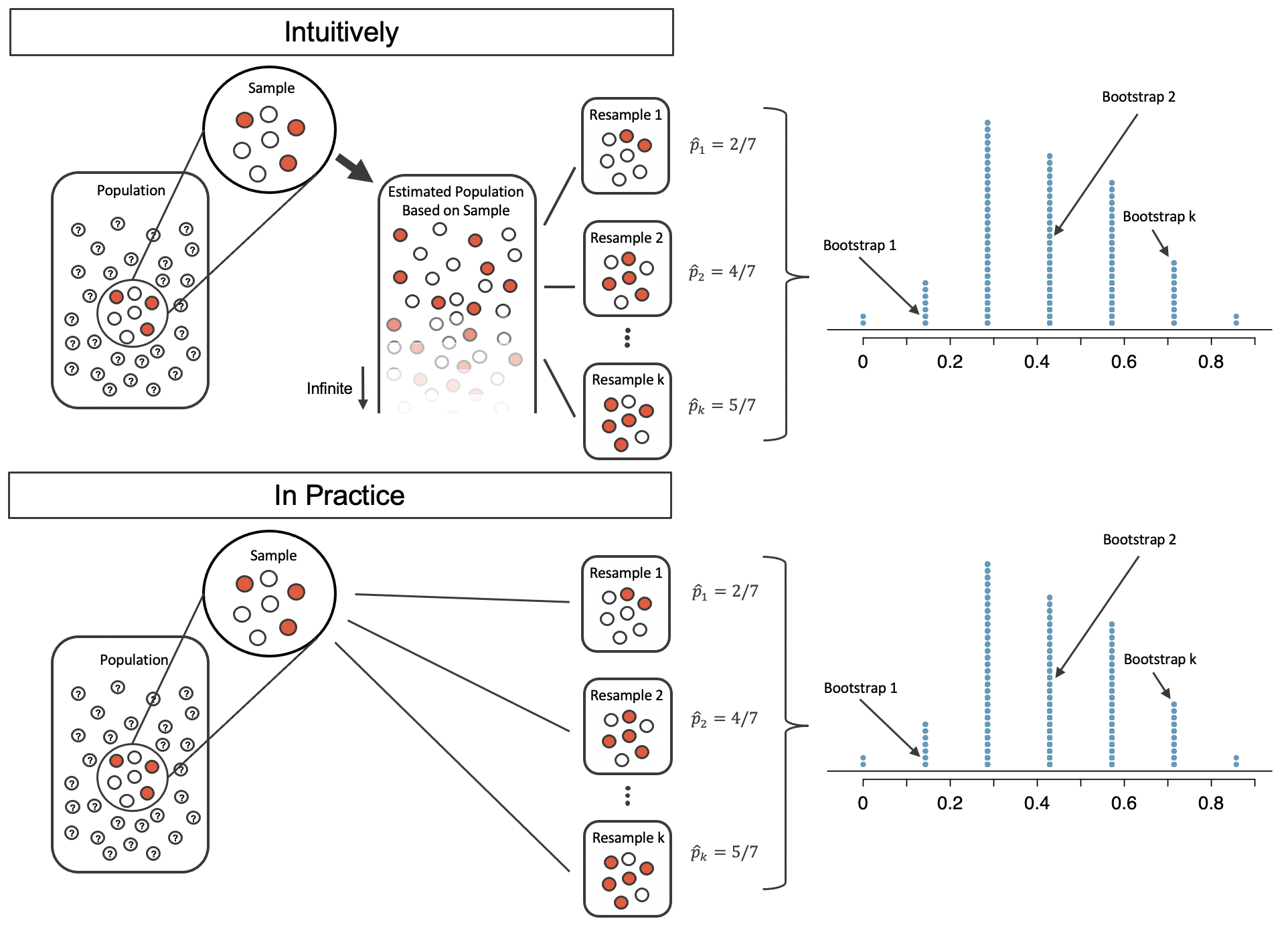
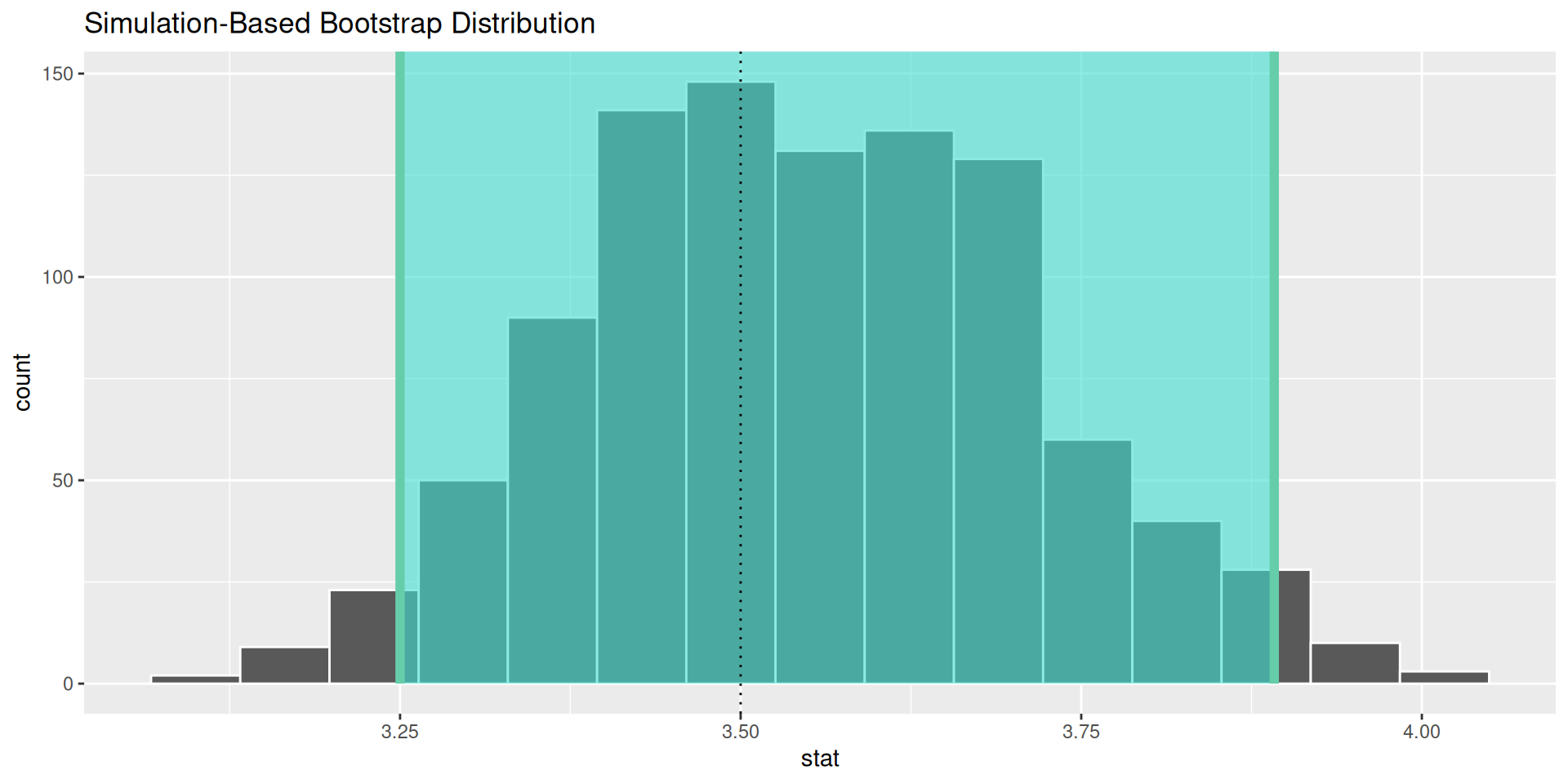
The bootstrap
Developed by Brad Efron in 1979
Resample from your sample with replacement!
Bootstrap distribution is similar to sampling distribution
The bootstrap distribution