Response: quarantine (factor)
# A tibble: 1 × 1
   stat
  <dbl>
1 0.820Confidence Intervals
IMS, Ch. 12
Smith College
Mar 10, 2026
Confidence intervals
Quantifying uncertainty
Small Idea
Our point estimate is the best single-number estimate of the population parameter (\(\mu_X\))
- Most often: the sample mean (\(\bar{x}\)) or proportion (\(\hat{p}\))
Big Idea
💡 We can use our understanding of the sampling distribution (of any random variable) to quantify our uncertainty surrounding this estimate
- This is better science
- But how do we construct the sampling distribution?
Your turn
See
help(ebola_survey)Use
specify()andcalculate()to compute the point estimate for the proportion of respondents favoring mandatory quarantine
How do we contruct the sampling distribution?
Method #1: calculate it using probability theory
- Model phenomenon and compute the sampling distribution
- Pros: exact
- Cons: requires strict assumptions, really hard to do in all but a few simple cases
- Take MTH 246 + MTH/SDS 320!
Method #2: approximate it using mathematical functions
- Use the CLT and (usually) the Normal distribution to approximate the sampling distribution
- Pros: works pretty well most of the time, well-known to statisticians, doesn’t require extensive computing power, deterministic
- Cons: not exact, requires assumptions, not always intuitive
- This is what your book calls “Mathematical model”
Method #3: simulate it using a computer
Use resampling techniques to construct the sampling distribution
- Pros: often relatively simple, easily generalizable, requires relatively modest assumptions
- Cons: non-deterministic, requires computing power
E.g., the bootstrap
Example
For a single proportion
- \(p\): the unknown true, fixed, population parameter
- \(\hat{p}\): the known, sample statistic…
- …but \(\hat{p}\) is a random variable
- subject to variability due to sampling
- it has a sampling distribution!
- Standard error (\(SE_{\hat{p}}\)): the standard deviation of the sampling distribution of \(\hat{p}\)
Bootstrap confidence interval
- Set \(\alpha = 0.05\)
- Percentile method: Cut off the top and bottom \(\alpha/2\) percentile of the bootstrap distribution
- Caveat: this doesn’t always work well
- There are other methods
Your turn
Use
generate()to construct a bootstrap distribution for \(\hat{p}\)Use
get_ci()to calculate a 95% CI for the proportion of respondents favoring mandatory quarantine
Interpreting confidence intervals
- Question: Does CI contain \(p\)?
- Answer:
YesorNo, but we will never know! - Compromise: can we make a statement about
probabilityhow likelyhow confident we are that the CI contains \(p\)?
Repeated sampling interpretation of confidence interval
A \(1-\alpha \%\) confidence interval for a population parameter will contain the true parameter \(1-\alpha \%\) of the time in repeated sampling
Misinterpretations are common
- \(p\) is unknown, and its value does not change
- The one sample proportion (\(\hat{p}\)) does not change either, and the confidence interval that you construct from it either will or will not contain the true mean (no chance involved)
- Your CI is for the true proportion: it doesn’t say anything about individual observations
- Always report \(p\)-values and a confidence interval
- Caveat: The margin of error represents a lower bound on the true uncertainty, for a variety of practical reasons
Interval width

Recall the analogy of the fisherman
Your turn
Use
visualize()to draw the sampling distribution of \(\hat{p}\)Use
shade_ci()to superimpose the CI on the sampling distribution
The result
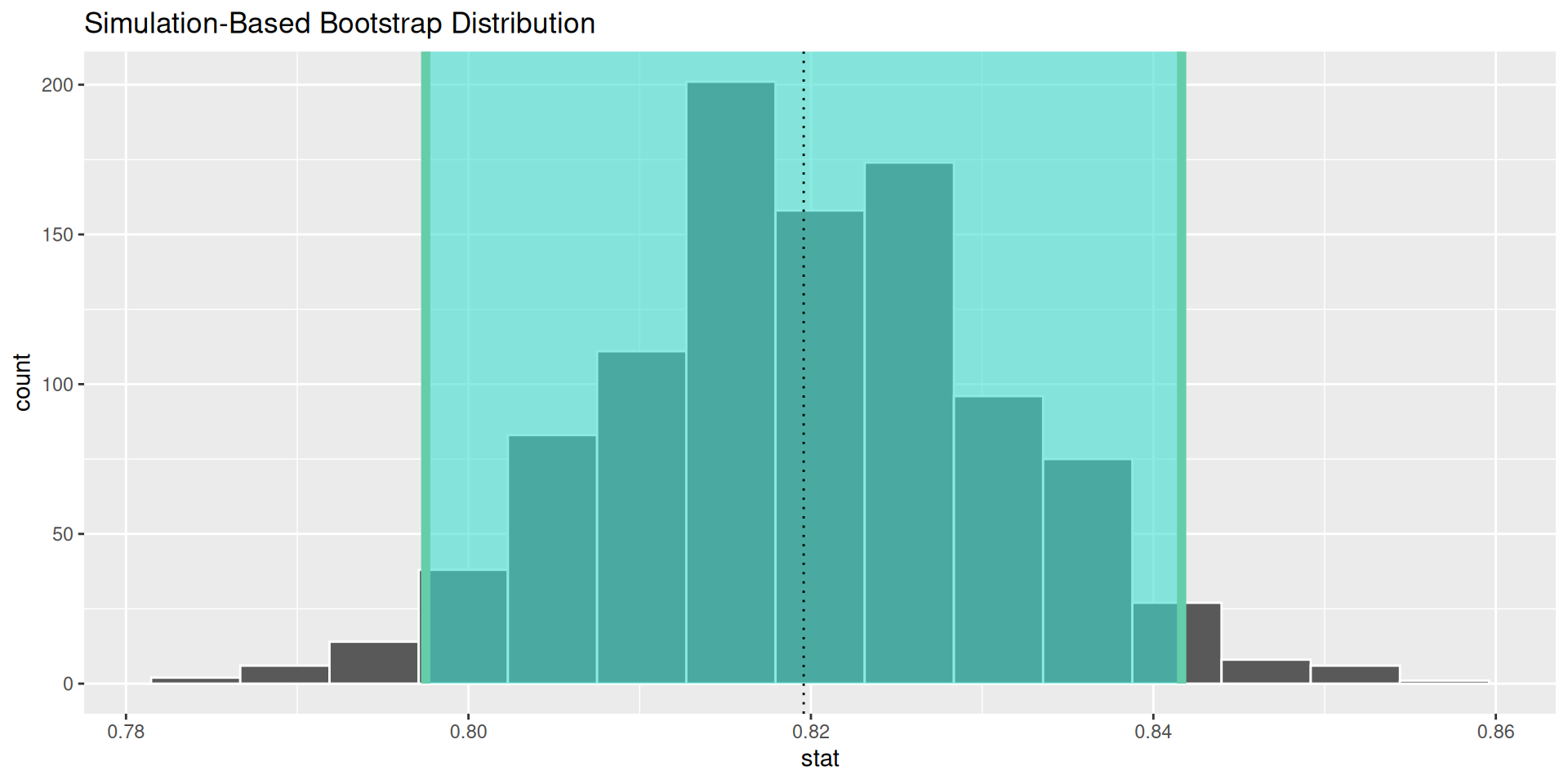
![]()