Inference for a single mean
IMS, Ch. 19
Smith College
Apr 15, 2026
Inference for a single mean
| Method | null dist. | sampling dist. |
|---|---|---|
| 1: probability | ?? | ?? |
| 2: simulation | ?? | bootstrap (centered at \(\bar{x}\)) |
| 3: \(t\)-approx. | \(\frac{\bar{x} - \mu_0}{s / \sqrt{n}} \sim t(d.f.)\) | \(\frac{\bar{x}}{s / \sqrt{n}} \sim t (d.f. )\) |
- See IMS, Chapter 19
UCLA book prices
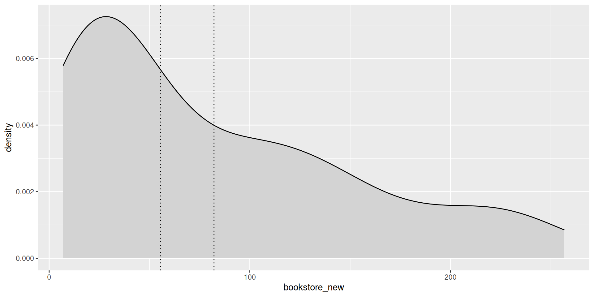
A sample of courses were collected from UCLA from Fall 2018, and the corresponding textbook prices were collected from the UCLA bookstore and also from Amazon.
Note
- Find a 95% confidence interval for the mean price of a textbook at the UCLA bookstore
Observed statistics
Distribution of book prices
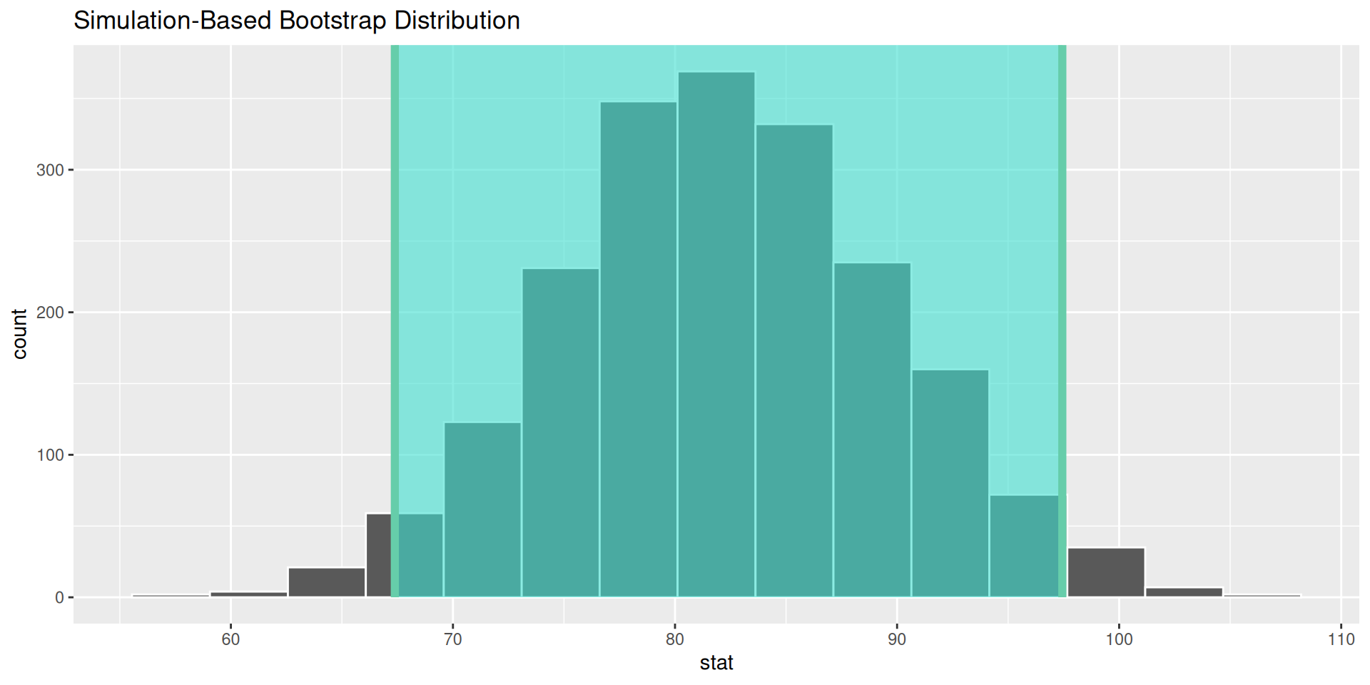
Method 2: Sampling distribution via bootstrap
Bootstrap distribution for mean
Confidence interval for the mean
Bootstrap distribution for median!
Confidence interval for a median
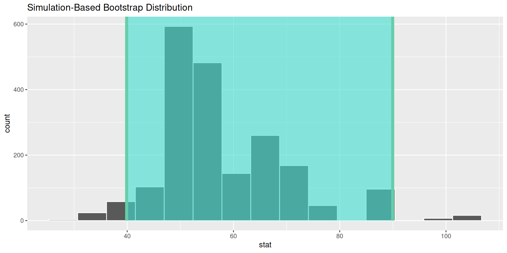
Note
We have no Central Limit Theorem for medians!
But the bootstrap should work anyway!
Method 3: Sampling distribution via approximation
Recall for a proportion
Let \(X \sim Bernoulli(p)\)
Then the sample proportion of \(n\) instances of \(X\) is: \[ \hat{p} = \frac{X_1 + \cdots + X_n}{n} \]
Binomial theory implies \[ Var(\hat{p}) = \frac{\hat{p} (1 - \hat{p})}{n} = \frac{Var(X)}{n} \]
So variance of sample proportion (a.k.a., the square of the standard error) is equal to variance of underlying r.v., divided by sample size
Now for a mean
Let \(X\) be a any r.v. Then, the sample mean of i.i.d. r.v.’s \(X_1, \ldots , X_n\) is: \[ \bar{x} = \frac{X_1 + \cdots + X_n}{n} \]
It follows that \[ Var(\bar{x}) = \frac{1}{n^2} \cdot n \cdot Var(X) = \frac{Var(X)}{n} \]
So variance of sample mean (a.k.a., the square of the standard error) is equal to variance of underlying r.v., divided by sample size
CLT
CLT implies that sampling distribution of \(\bar{x}\) approaches normal as \(n \rightarrow \infty\)
But we don’t know \(Var(X) \equiv \sigma_X^2\)!!
We have to estimate \(\sigma_X\) with \(s_X\) (the sample standard deviation)
This introduces extra uncertainty
Statisticians have shown that this extra uncertainty is captured by the \(t\)-distribution (rather than the Normal)
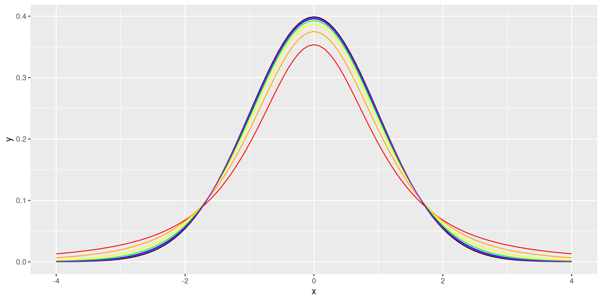
\(t\)-distribution
- Like the standard normal but with fatter tails
- 1 parameter: d.f.
t_plot <- ggplot() +
  stat_function(fun = dnorm, fill = "darkgray") +
  lims(x = c(-4, 4)) +
  stat_function(fun = dt, args = list(df = 2), color = "red") +
  stat_function(fun = dt, args = list(df = 4), color = "orange") +
  stat_function(fun = dt, args = list(df = 8), color = "yellow") +
  stat_function(fun = dt, args = list(df = 16), color = "green") +
  stat_function(fun = dt, args = list(df = 32), color = "blue") +
  stat_function(fun = dt, args = list(df = 64), color = "purple")
It looks like this
How do we use it?
- \(t^*_{\alpha/2}\):
- Margin of error: \(t^*_{\alpha/2} \cdot SE_{\bar{x}}\)
- Confidence Interval: \(\bar{x} \pm t^*_{\alpha/2} \cdot SE_{\bar{x}}\)
Book prices
- Standard error
Book prices
- Confidence interval
[1] 14.75066[1] 67.39214 96.89347Your turn
See handout
![]()