# A tibble: 2 × 4
  location       num_days mean_kwh sd_kwh
  <chr>             <int>    <dbl>  <dbl>
1 Haight_Ashbury      215    38.6   19.1
2 Inner_Sunset 69 9.01 4.86Inference for many means
IMS, Ch. 22
Smith College
Nov 16, 2022
Paired t-test
Paired t-test
Your data is naturally paired if:
- you have \(n\) observations of variables \(X\) and \(Y\)
- \(X_i\) naturally corresponds to \(Y_i\)
- interested in testing if \(X\) is different than \(Y\)
- What to do?
- Compute \(D_i = X_i - Y_i\)
- Set \(H_0: \mu_0 = 0\)
- Proceed with inference for a single mean
- See IMS, Chapter 21
Quick example: Energy Output
The data provide the energy output for several months from two roof-top solar arrays in San Francisco. This city is known for having highly variable weather, so while these two arrays are only about 1 mile apart from each other, the Inner Sunset location tends to have more fog.
Data space
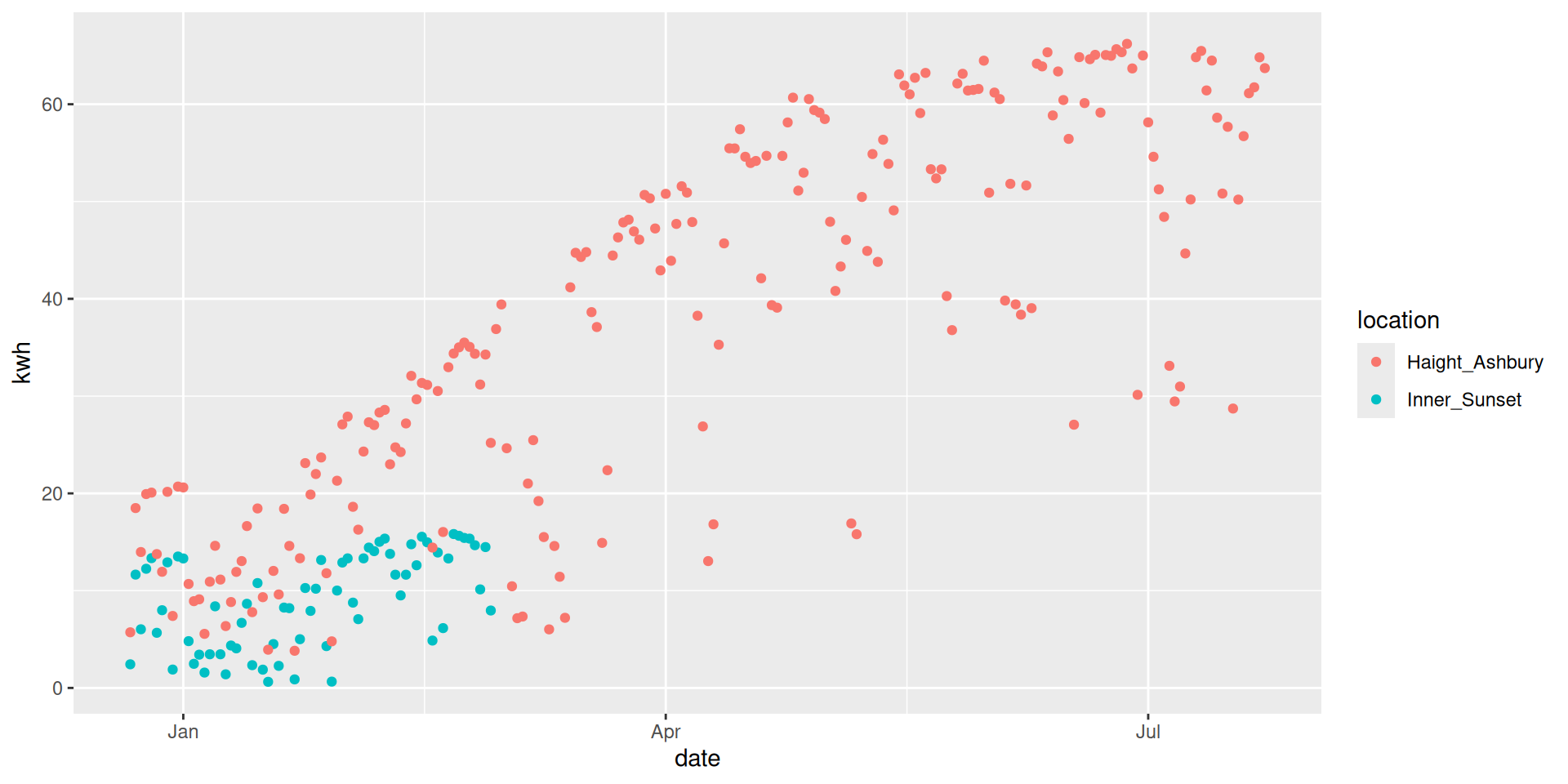
Natural pairing by date
# A tibble: 69 × 4
   date       Inner_Sunset Haight_Ashbury  diff
   <date>            <dbl>          <dbl> <dbl>
 1 2015-12-22         2.43           5.72  3.29
 2 2015-12-23        11.6           18.5   6.84
 3 2015-12-24         6.03          14.0   7.94
 4 2015-12-25        12.2           19.9   7.68
 5 2015-12-26        13.3           20.1   6.74
 6 2015-12-27         5.67          13.8   8.09
 7 2015-12-28         7.99          11.9   3.95
 8 2015-12-29        12.9           20.2   7.25
 9 2015-12-30         1.89           7.4   5.51
10 2015-12-31        13.5           20.7   7.19
# ℹ 59 more rows
Paired test vs. two-sample test
# A tibble: 1 × 7
  statistic  t_df  p_value alternative estimate lower_ci upper_ci
      <dbl> <dbl>    <dbl> <chr>          <dbl>    <dbl>    <dbl>
1      8.37  103. 3.05e-13 two.sided       10.5     8.01     13.0
# A tibble: 1 × 7
statistic t_df p_value alternative estimate lower_ci upper_ci
<dbl> <dbl> <dbl> <chr> <dbl> <dbl> <dbl>
1 17.4 68 1.13e-26 two.sided 10.5 9.29 11.7ANOVA
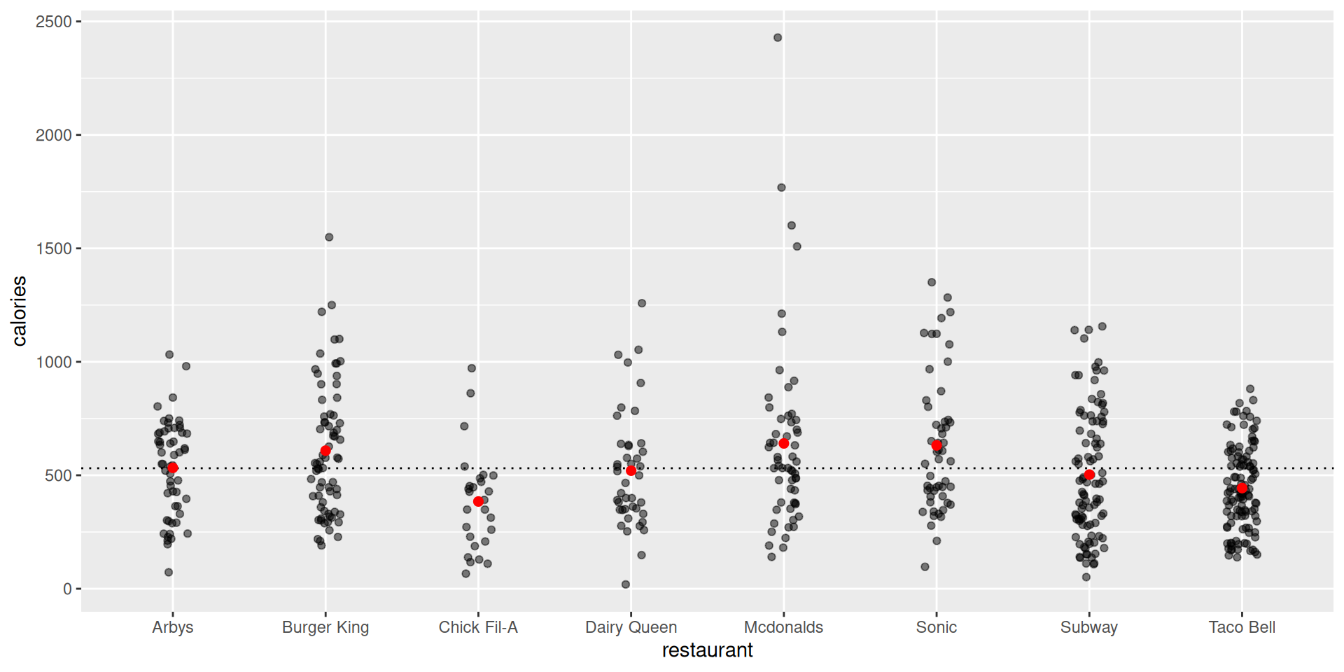
Calories across fast food restaurants
Nutrition amounts in 515 fast food items. Are there meaningful differences across different chains?
# A tibble: 8 × 4
  restaurant  num_items mean_calories sd_calories
  <chr>           <int>         <dbl>       <dbl>
1 Arbys              55          533.        210.
2 Burger King        70          609.        290.
3 Chick Fil-A        27          384.        220.
4 Dairy Queen        42          520.        259.
5 Mcdonalds          57          640.        411.
6 Sonic              53          632.        301.
7 Subway             96          503.        282.
8 Taco Bell         115          444.        184.
Data space
How to proceed
What if we did \(\binom{8}{2} = 28\) two-sample t-tests?
How many false positives would we expect?
Why is this comic funny? http://xkcd.com/882/
ANOVA as things you already know
One-way ANOVA is just regression with a numerical response variable and a single categorical explanatory variable
A two-sample t-test is just a special case of ANOVA where there are only two groups
ANOVA formulations
- Consider the following formulations of the same model:
\[ \begin{align*} y_{ij} &= \mu_i + \epsilon_{ij}, \text{ where } \epsilon_{ij} \sim N(0, \sigma) \\ y_{ij} &= \mu + \alpha_i + \epsilon_{ij}, \text{ where } \epsilon_{ij} \sim N(0, \sigma) \\ y_{ij} &= \mu_1 + \beta_i \cdot X_i + \epsilon_{ij}, \text{ where } \epsilon_{ij} \sim N(0, \sigma) \end{align*} \] for groups \(i = 1,\ldots, I\) and individuals \(j=1,\ldots,n_i\), with common standard deviation \(\sigma\).
Model 1: group means
Tables of means
Grand mean

530.9126

 restaurant
    Arbys Burger King Chick Fil-A Dairy Queen Mcdonalds Sonic Subway Taco Bell
    532.7       608.6       384.4       520.2     640.4 631.7    503     443.7
rep 55.0 70.0 27.0 42.0 57.0 53.0 96 115.0- \(\mu_i\)’s are the group means
- Note grand mean (\(\mu\)) in output!
Model 2: grand mean + group effects
Tables of effects

 restaurant
     Arbys Burger King Chick Fil-A Dairy Queen Mcdonalds Sonic Subway Taco Bell
     1.815       77.66      -146.5      -10.67     109.4 100.8 -27.89    -87.26
rep 55.000 70.00 27.0 42.00 57.0 53.0 96.00 115.00- \(\mu\) is the grand mean
- \(\alpha_i\)’s are the group effects
Model 3: regression
# A tibble: 8 × 5
  term                  estimate std.error statistic  p.value
  <chr>                    <dbl>     <dbl>     <dbl>    <dbl>
1 (Intercept)              533.       36.8    14.5   6.01e-40
2 restaurantBurger King     75.8      49.2     1.54  1.24e- 1
3 restaurantChick Fil-A   -148.       64.2    -2.31  2.13e- 2
4 restaurantDairy Queen    -12.5      56.0    -0.223 8.24e- 1
5 restaurantMcdonalds      108.       51.6     2.08  3.76e- 2
6 restaurantSonic           99.0      52.6     1.88  6.03e- 2
7 restaurantSubway         -29.7      46.2    -0.643 5.20e- 1
8 restaurantTaco Bell -89.1 44.8 -1.99 4.72e- 2- \(\beta_i\)’s are the group effects relative to the reference group
- Reference group is the first factor level (alphabetical by default)
Grand mean
- Estimate of grand mean \(\mu\) with \(\hat{y}\)
Compare model coefficients
# mu_i's
group_means <- model.tables(mod_anova, "means")$tables$restaurant
# alpha_i's
group_effects <- model.tables(mod_anova, "effects")$tables$restaurant
# beta_i's
group_refs <- broom::tidy(mod_lm)$estimate |>
    set_names(nm = names(group_means))
tibble(
  restaurant = names(group_means),
  group_means, group_effects, group_refs
)
# A tibble: 8 × 4
restaurant group_means group_effects group_refs
<chr> <mtable[1d]> <mtable[1d]> <dbl>
1 Arbys 532.7273 1.814651 533.
2 Burger King 608.5714 77.658807 75.8
3 Chick Fil-A 384.4444 -146.468177 -148.
4 Dairy Queen 520.2381 -10.674526 -12.5
5 Mcdonalds 640.3509 109.438256 108.
6 Sonic 631.6981 100.785492 99.0
7 Subway 503.0208 -27.891788 -29.7
8 Taco Bell 443.6522 -87.260447 -89.1$`Grand mean`
[1] 530.9126The models are the same!
Because:
- \(\hat{y}_{ij}\)’s are all the same
- \(\hat{\epsilon}_{ij}\)’s are all the same
But are the observed differences meaningful?
Let’s do a hypothesis test!
Partitioning variability
- The sum of squares and degrees of freedom are partitioned as \[ \begin{align*} SS_{Total} &= SS_{Groups} + SS_{Residuals} \\ d.f._{Total} &= d.f._{Groups} + d.f._{Residuals} \end{align*} \]
F-test
- null hypotheses (equivalent):
- \(\mu_i = \mu_j\) for all \(i, j\)
- \(\alpha_i = 0\) for all \(i=1,\ldots,I\)
- \(\beta_i = 0\) for all \(i=1,\ldots,I-1\)
- test statistic:
\[ F = \frac{SS_{Groups} / d.f._{Groups}}{SS_{Residuals} / d.f._{Residuals}} \]
F-test (continued)
Test statistic follows an F-distribution
\(d.f._{Groups} = \text{number of factor levels} - 1\)
\(d.f._{Residuals} = n - d.f._{Groups}\)
F-test in R
Analysis of Variance Table

Response: calories
            Df   Sum Sq Mean Sq F value    Pr(>F)
restaurant   7  3177729  453961   6.085 7.747e-07 ***
Residuals  507 37824143   74604
---
Signif. codes: 0 '***' 0.001 '**' 0.01 '*' 0.05 '.' 0.1 ' ' 1Null distribution
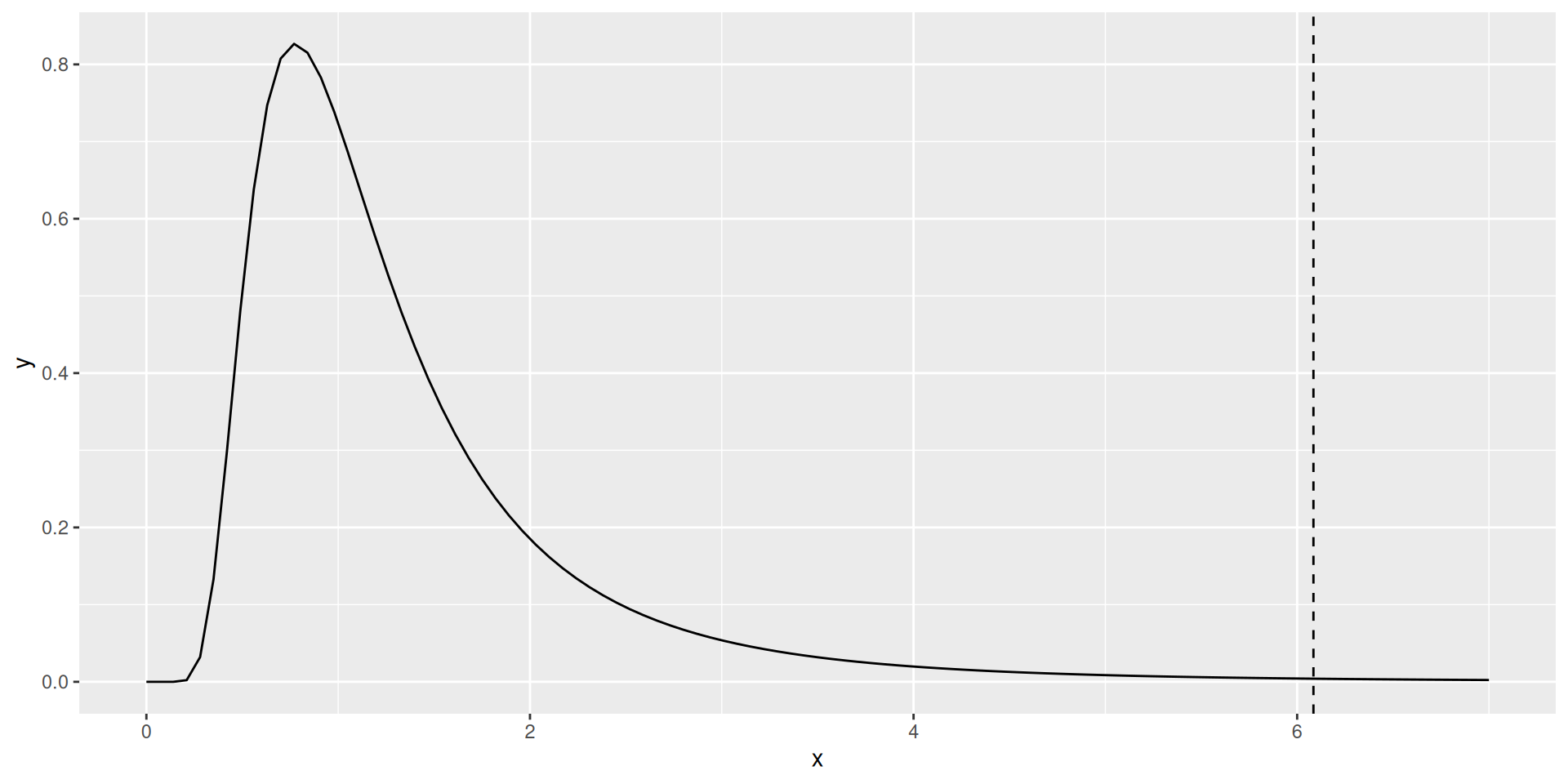
Conclusion
We reject the null hypothesis that the mean number of calories among food items are the same for all eight restaurants.
Thus, there is a statistically significant difference in the average number of calories per item on the menu across eight different fast food restaurants.
More sophisticated testing procedures are necessary to determine how many, and which, restaurants differ from each other.
Your turn
See handout
Multiple testing
Combating multiple comparisons
Simplest (and most conservative):
- Bonferroni’s correction:
- simply divide the \(\alpha\)-level by the number of comparisons
Other approaches: