# A tibble: 6 × 13
   fage  mage mature      weeks premie visits gained weight lowbirthweight sex
  <int> <dbl> <chr>       <dbl> <chr>   <dbl>  <dbl>  <dbl> <chr>          <chr>
1    34    34 younger mom    37 full …     14     28   6.96 not low        male
2    36    31 younger mom    41 full …     12     41   8.86 not low        fema…
3    37    36 mature mom     37 full …     10     28   7.51 not low        fema…
4    NA    16 younger mom    38 full …     NA     29   6.19 not low        male
5    32    31 younger mom    36 premie     12     48   6.75 not low        fema…
6    32    26 younger mom    39 full …     14     45   6.69 not low        fema…
# ℹ 3 more variables: habit <chr>, marital <chr>, whitemom <chr>Inference for regression (bootstrap)
IMS, Ch. 24
Nov 21, 2022
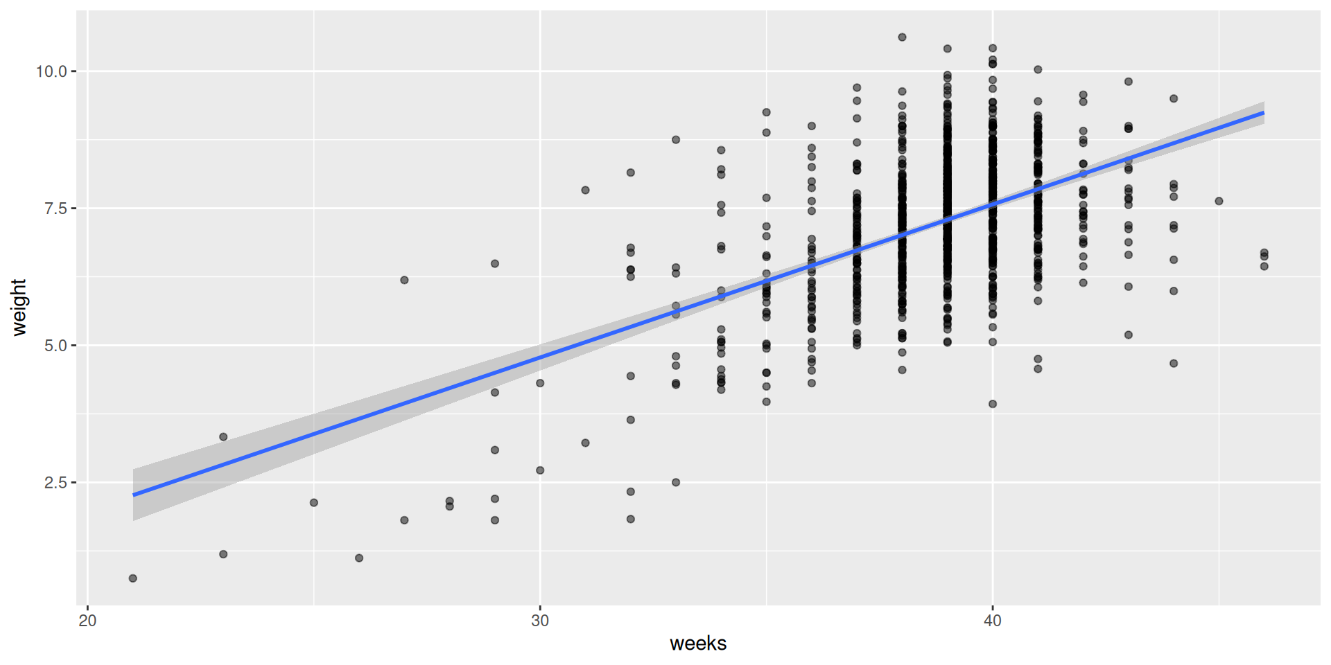
Data space
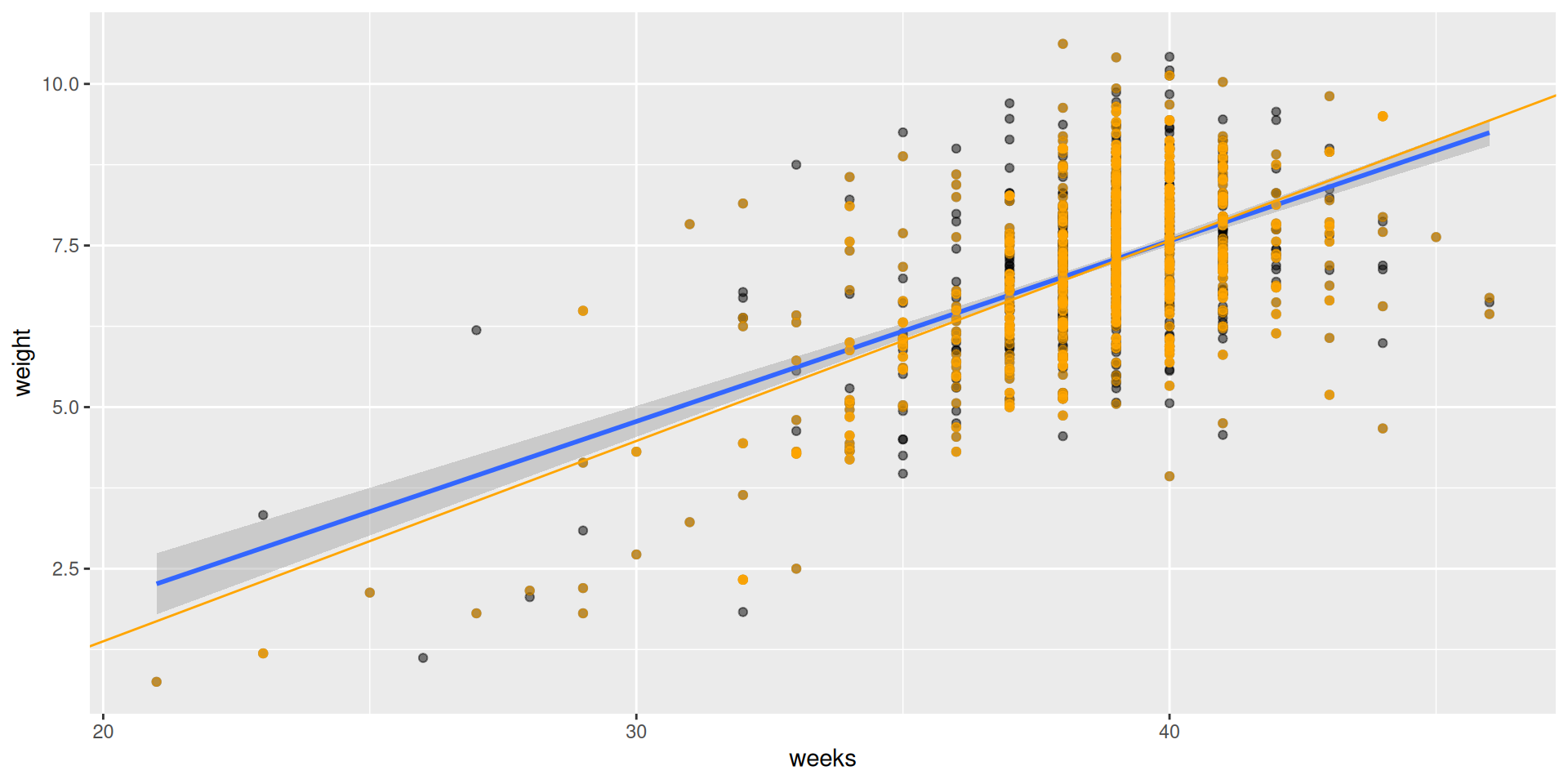
Resample in the data space
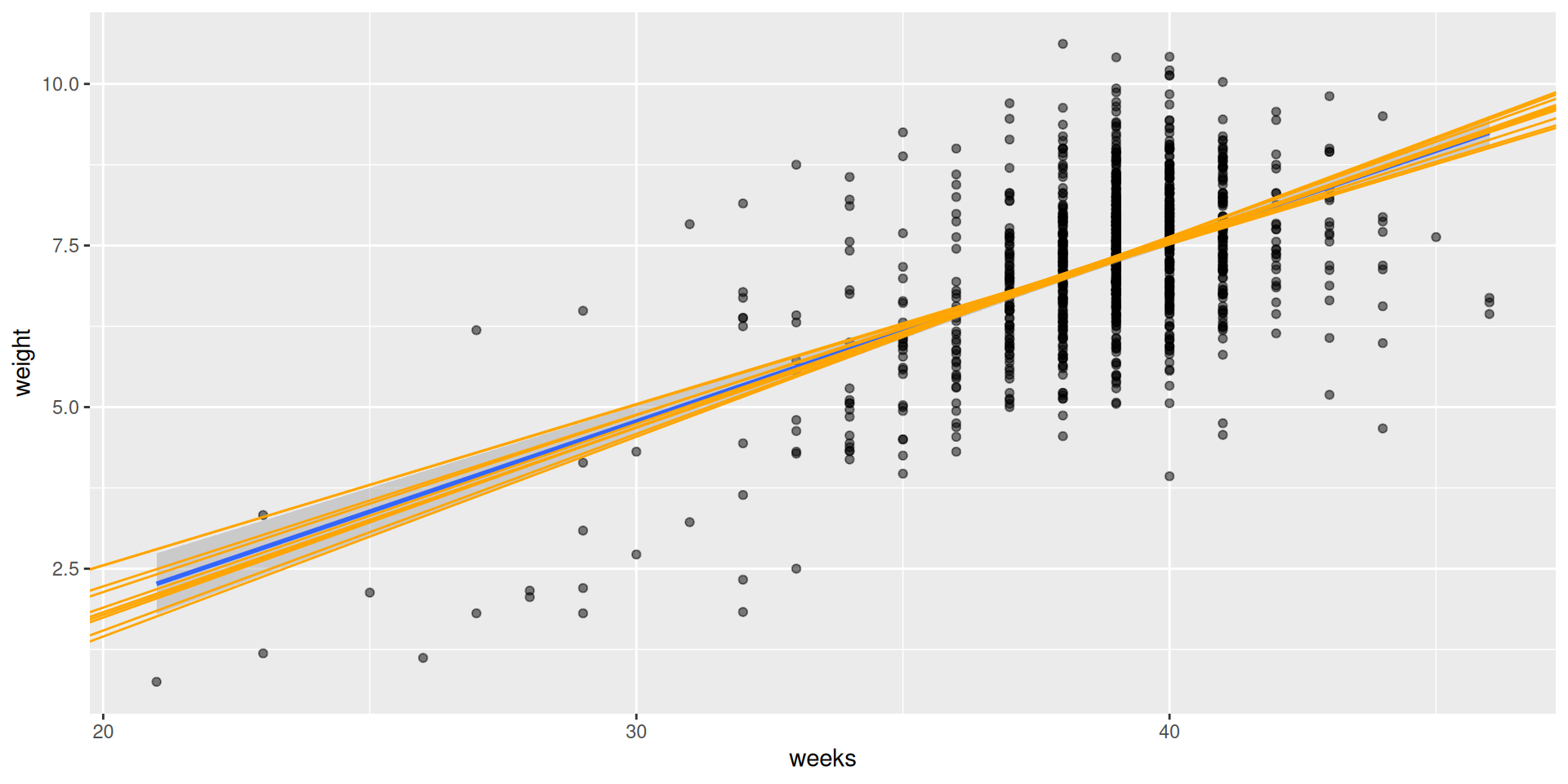
Many resamples in the data space
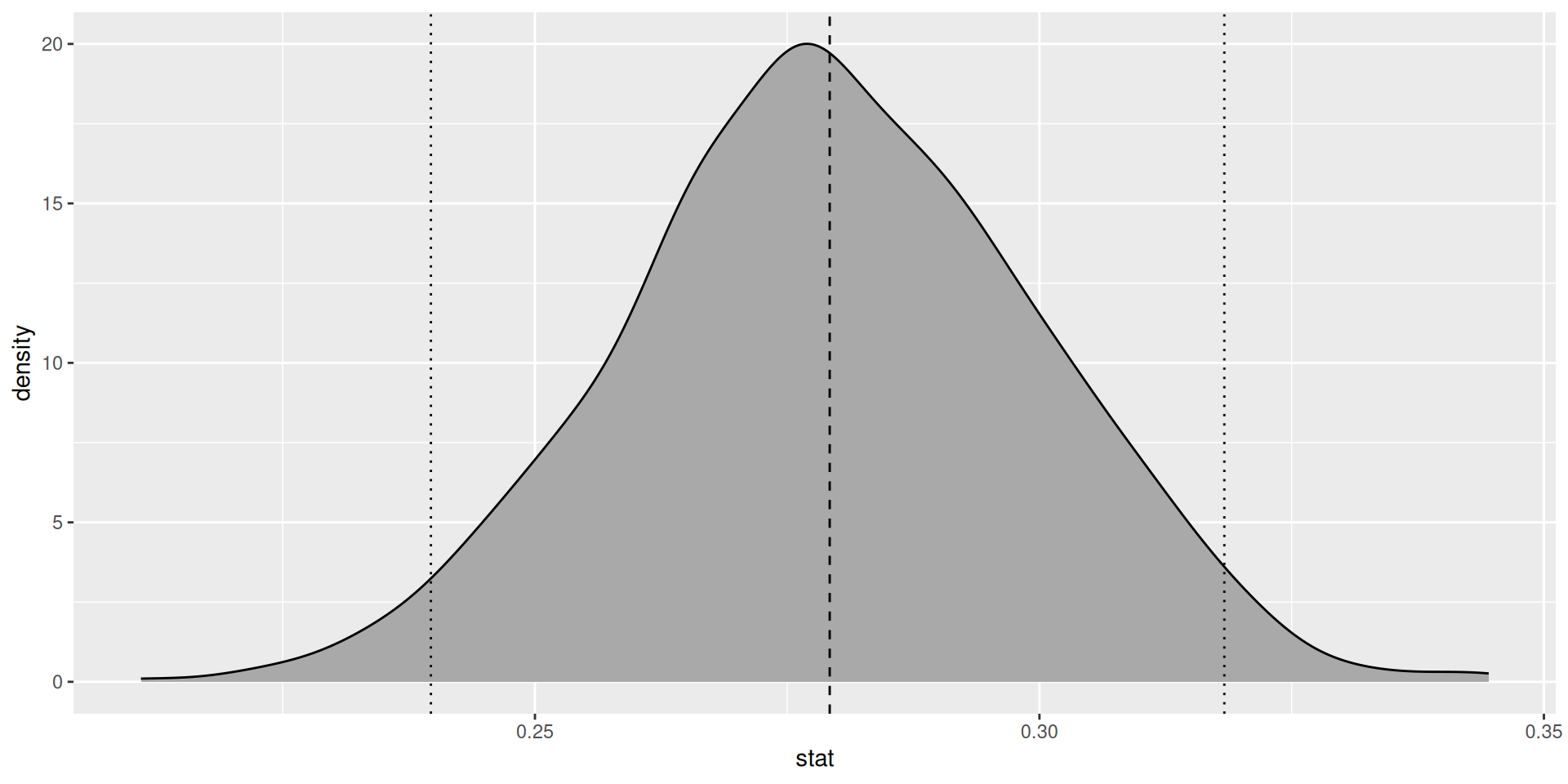
Sampling distribution of the slope