02-Simple Linear Regression
SDS 291
September 10, 2025
Recap: Statistical modeling
Form of a statistical model
\[ \text{Observed data} = \text{mathematical model} + \text{random error} \]
\[ \underbrace{y}_{\text{response}} = \underbrace{f}_{\text{model}}( \underbrace{x}_{\text{explanatory}}) + \underbrace{\epsilon}_{\text{error}} \]
Pieces of a statistical model
- Mathematical model
- Deterministic mathematical function
- Encodes our assumptions about true signal in our data
- e.g., the mean (expected value) of the outcome
- Random error
- Random variable
- Encodes our assumptions about the noise in our data
- e.g., “white noise” or static
Signal vs. Noise

Goals of Building a Statistical Model
- Summarize a pattern observed in data
- Goal: descriptive
- Predict values of the response
- Goal: Inferential
- Quantify the strength of relationships among variables
- Goal: Inferential
Note
Today: summarizing linear patterns in the data! 🎉
The Vietnam War Draft of 1969
Draft numbers
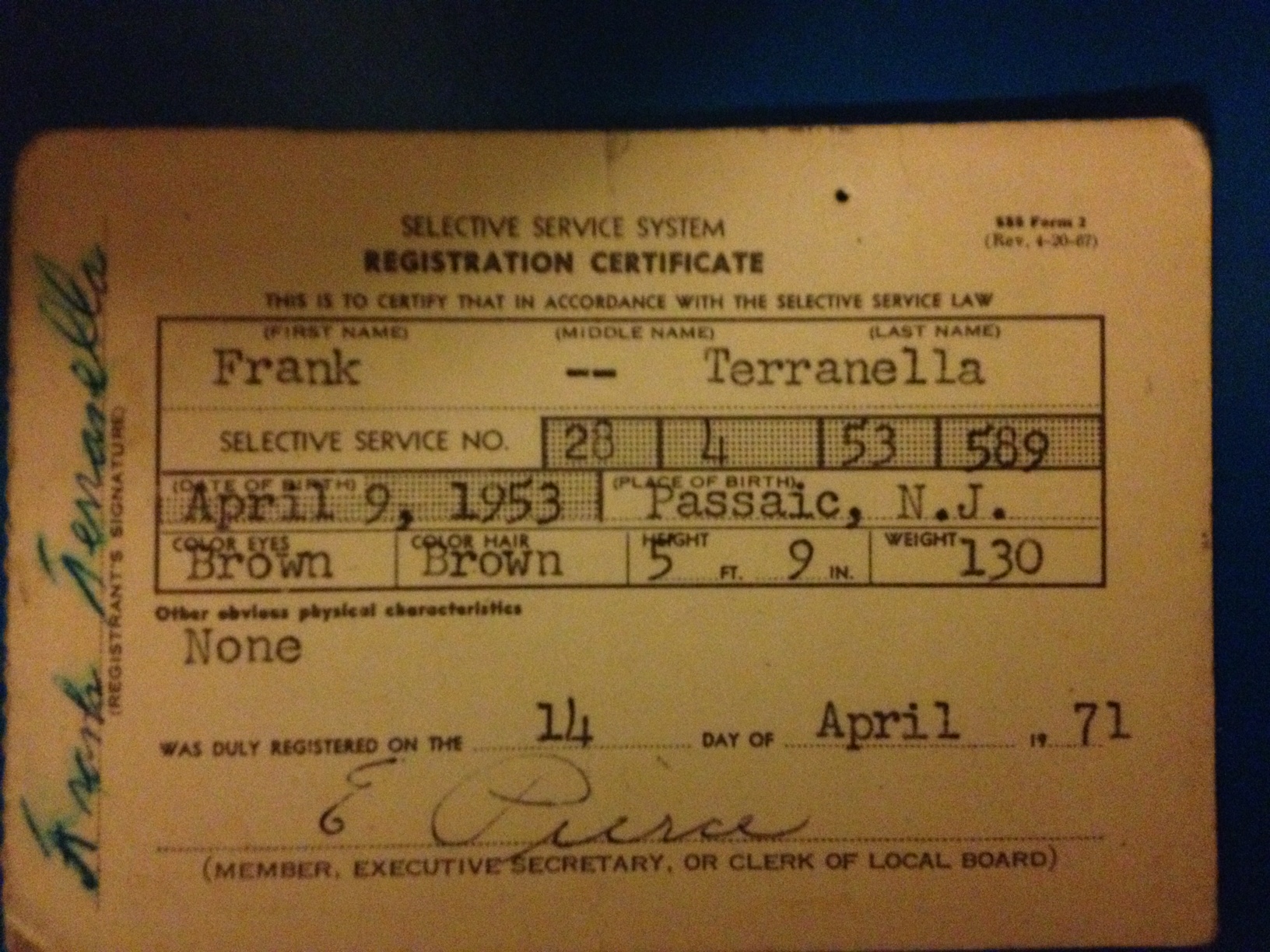
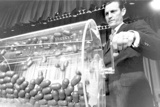
The Vietnam War Draft of 1969
- Sample: the data that we have in hand
- Observational units: what we take measurements on
- Variables: what we measure
The Vietnam draft data
# A tibble: 6 × 6
  month   day min_year max_year day_rank draft_number
  <dbl> <dbl>    <dbl>    <dbl>    <dbl>        <dbl>
1     1     1     1944     1950        1          305
2     1     2     1944     1950        2          159
3     1     3     1944     1950        3          251
4     1     4     1944     1950        4          215
5     1     5     1944     1950        5          101
6 1 6 1944 1950 6 224What pattern(s) do you see?
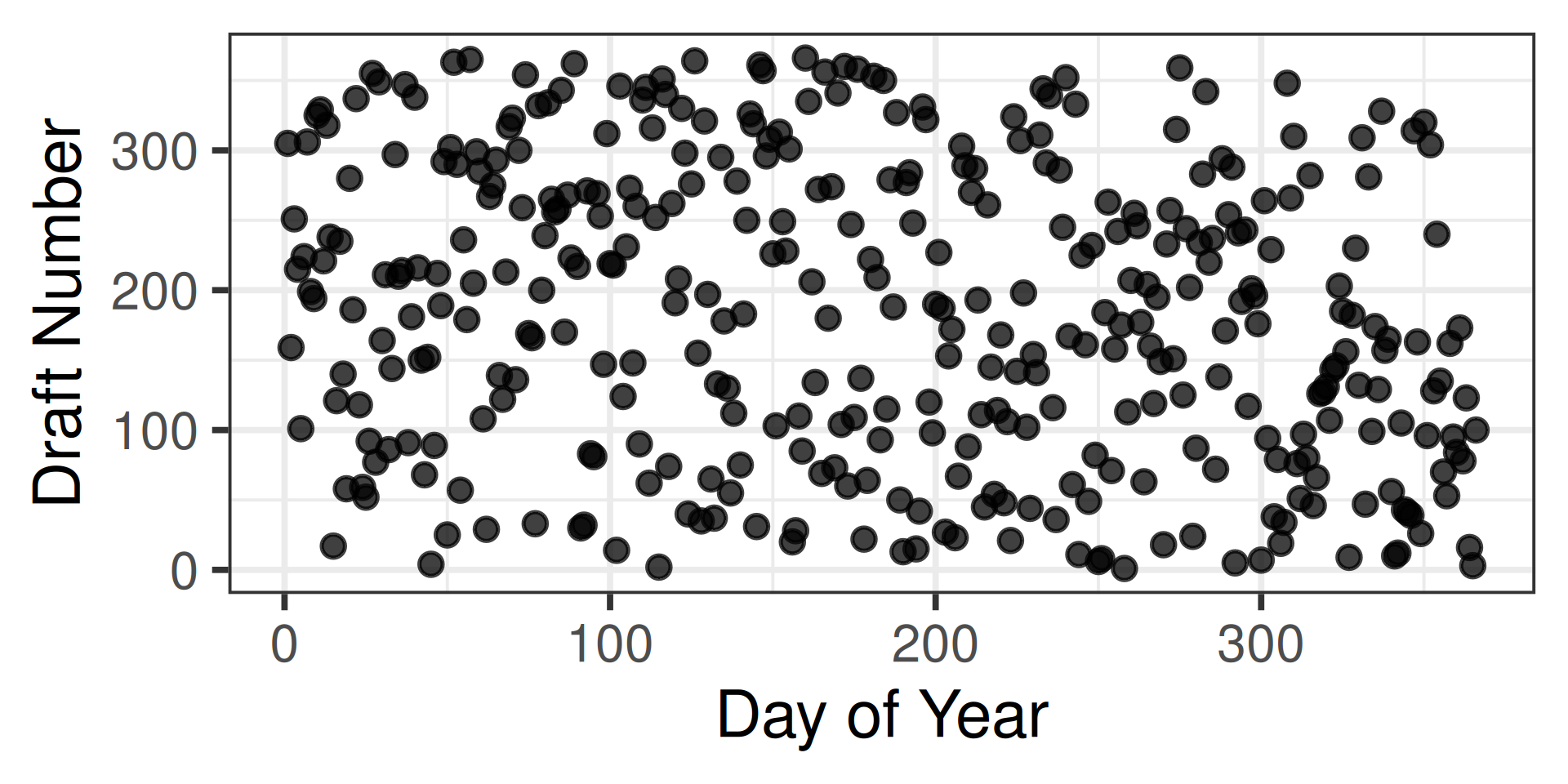
- Form? (linear, quadratic, sinusoidal, etc.)
- Direction? (increasing or decreasing?)
- Strength? (random error: a lot or a little?)
The null model
The mean as a statistical model
Tip
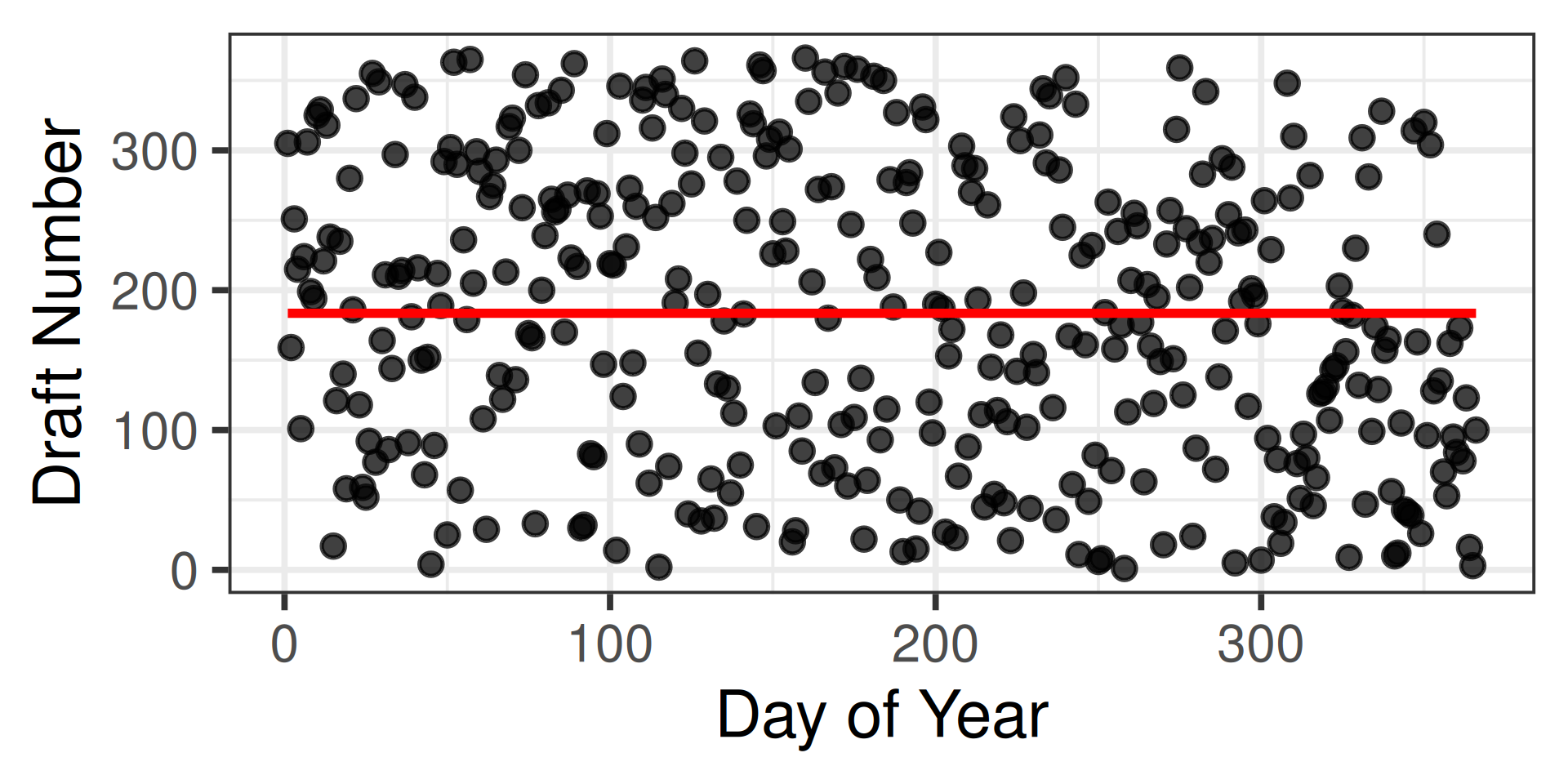
Assumption: average value of the response is the same for all observations, regardless of the value of the explanatory variable
For each ball in the glass jar (\(i = 1, \ldots, n\)),
\[ \underbrace{\ y_{i}\ }_{\substack{\text{actual} \\ \text{draft no.}}} = \underbrace{\ \mu\ }_{\substack{\text{mean} \\ \text{draft no.}}} + \underbrace{\ \epsilon_{i}\ }_{\substack{\text{random} \\ \text{error}}} \]
Visualizing the null model
Fitting the null model
Tip
“Fitting a model” refers to estimating the parameters in the model (in this case, \(\mu\))
\[\begin{align*} \widehat{\mu} &= \frac{1}{n}\sum_{i=1}^{n}y_i \\ &= \frac{1}{n}(y_1 + y_2 + \cdots + y_n) \\ &= \bar{y} \end{align*}\]
Estimating the mean
The Data:
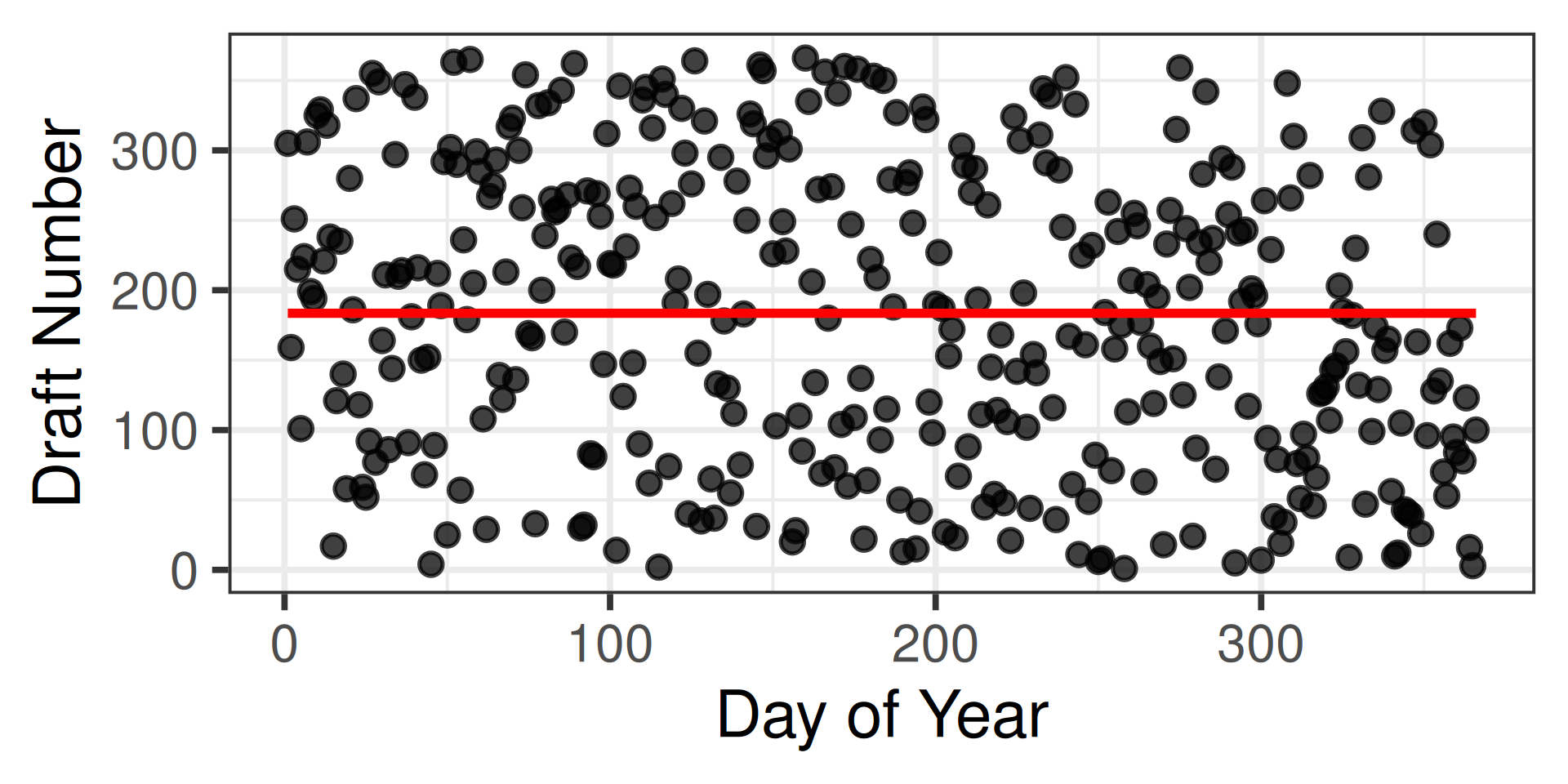
The Fitted Model:
\[\begin{align*} \widehat{\mu} &= \frac{1}{n}\sum_{i=1}^{n}y_i \\ &= \frac{1}{n}(y_1 + y_2 + \cdots + y_n) \\ &= \frac{1}{n}(1 + 2 + \cdots + 366) \\ &= 183.5 \end{align*}\]
Fitting the model in R
Call:
lm(formula = draft_number ~ 1, data = draft_data)

Coefficients:
(Intercept)
183.5 Capturing the leftover variability
- residual (\(e_i\)): difference between the observed value of the response and the fitted value
\[\begin{align*} e_i &= \text{observed} - \text{fitted}\\ &= y_i - \hat{y}_i \end{align*}\]
Computing the residuals
Tip
- The residual (\(e_i\)) is an estimate of the random error term \(\epsilon_i\)
# A tibble: 366 × 7
   draft_number .fitted .resid    .hat .sigma   .cooksd .std.resid
          <dbl>   <dbl>  <dbl>   <dbl>  <dbl>     <dbl>      <dbl>
 1          305    183.  122.  0.00273   106. 0.00362       1.15
 2          159    183.  -24.5 0.00273   106. 0.000147     -0.232
 3          251    183.   67.5 0.00273   106. 0.00112       0.639
 4          215    183.   31.5 0.00273   106. 0.000244      0.298
 5          101    183.  -82.5 0.00273   106. 0.00167      -0.781
 6          224    183.   40.5 0.00273   106. 0.000403      0.383
 7          306    183.  123.  0.00273   106. 0.00368       1.16
 8          199    183.   15.5 0.00273   106. 0.0000590     0.147
 9          194    183.   10.5 0.00273   106. 0.0000271     0.0994
10          325    183.  142.  0.00273   106. 0.00491       1.34
# ℹ 356 more rows
Simple linear regression
A straight line model
Tip
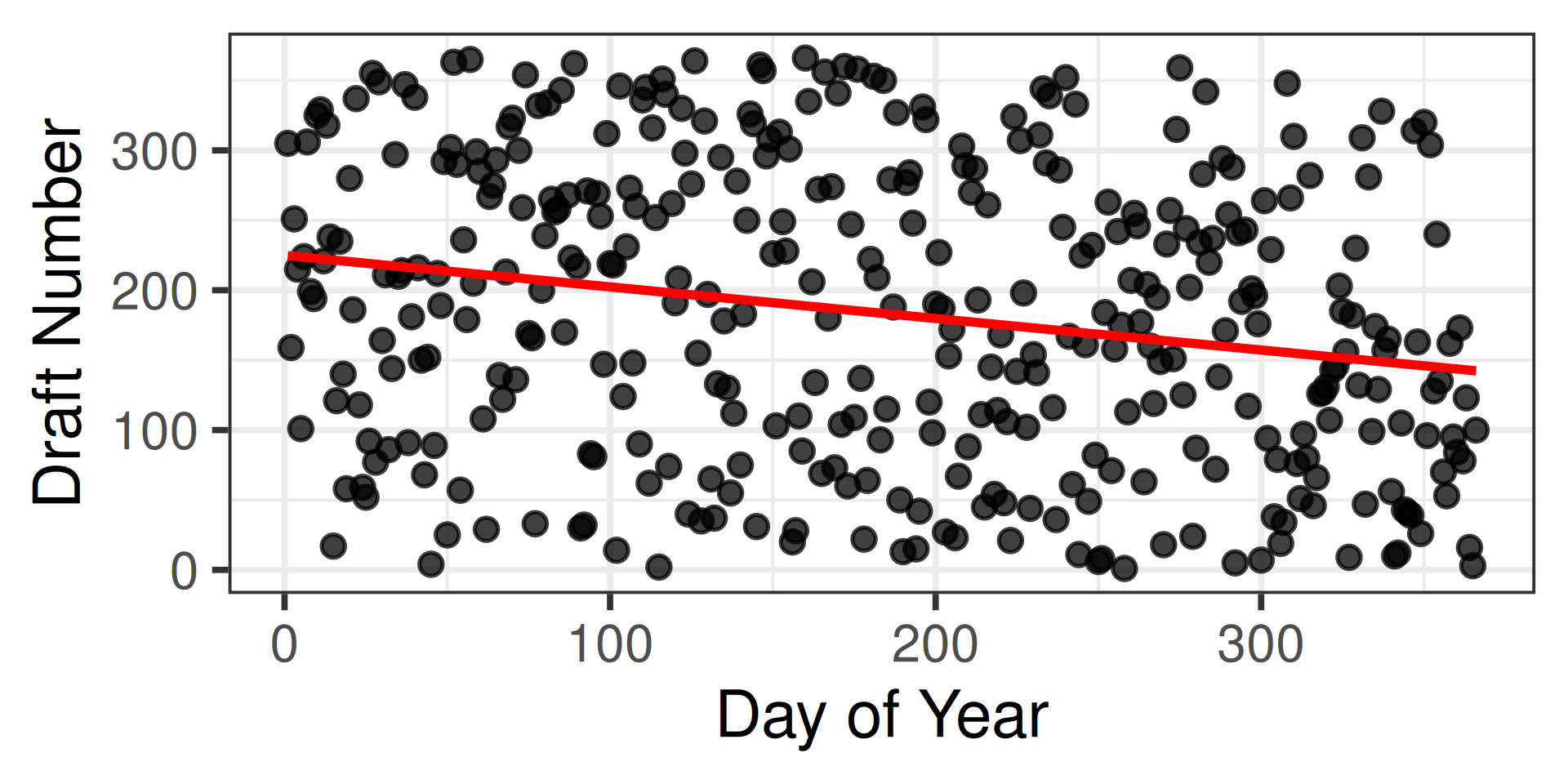
Assumption: average value of the response depends on the explanatory variable in a linear fashion
- For a ball with a birthday \(x_i\) days after the start of the year,
\[ \underbrace{\ y_{i}\ }_{\substack{\text{actual} \\ \text{draft no.}}} = \underbrace{\ \beta_0 + \beta_1 \cdot x_i \ }_{\substack{\text{mean} \\ \text{draft no.}\\ \text{for that day}}} + \underbrace{\ \epsilon_{i}\ }_{\substack{\text{random} \\ \text{error}}} \]
Visualizing the SLR model
It’s like Greek to me
- In statistics, we write quantities of interest that are unknown to us with Greek letters (like \(\beta\) or \(\mu\))
- \(\beta_0\) represents the unknown intercept
- \(\beta_1\) represents the unknown slope
- We use hats (\(\hat{\mu}\)) to denote known estimates of the corresponding unknown Greek quantities!
- \(\hat{\beta}_0\) represents the known fitted intercept
- \(\hat{\beta}_1\) represents the known fitted slope
Statistical model (unknown parameters):
\[\begin{align*} Y &= \underbrace{\beta_0 + \beta_1 \cdot X}_{signal} + \underbrace{\epsilon}_{noise} \, (\text{random variables}) \\ \mathbb{E}[Y | X] &= \underbrace{\beta_0 + \beta_1 \cdot X}_{signal} + \underbrace{\epsilon}_{noise} \, (\text{expected value}) \\ y_i &= \underbrace{\beta_0 + \beta_1 \cdot x_i}_{signal} + \underbrace{\epsilon_i}_{noise} \, (\text{individual observation}) \end{align*}\]
Fitted model (estimated parameters)
\[\begin{align*} \widehat{Y} &= \hat{\beta}_0 + \hat{\beta}_1 \cdot X \, (\text{random variables}) \\ \widehat{y}_i &= \hat{\beta}_0 + \hat{\beta}_1 \cdot x_i \, (\text{individual observation}) \end{align*}\]
Interpretation of intercept (\(\beta_0\))
- y-intercept
- expected value of \(Y\) when \(x=0\)
- The expected value of the response variable among the observational units with an explanatory variable value of 0 units is \(\beta_0\) units
Interpretation of slope (\(\beta_1\))
- slope
- expected change in \(Y\) when \(x\) increases by one unit
- A one unit increase in the explanatory variable is associated with a \(\beta_1\) unit change in the expected value of the response variable
Ordinary least squares (OLS)
Note
Find the values \(\hat{\beta}_0\) and \(\hat{\beta}_1\) that will minimize the squared discrepancy between the data and the fitted model for the mean
- Find \(\hat{\beta}_0\) and \(\hat{\beta}_1\) that minimize
\[ SSE = \sum_{i=1}^{n}e_i^2 = \sum_{i=1}^{n} \left( y_i - \underbrace{\left( \hat{\beta}_0 + \hat{\beta}_1 x_i \right)}_{\hat{y}_i} \right)^2 \]
Statisticians have proven that
- The optimal slope coefficient is:
\[\begin{align*} \hat{\beta}_1 &= \frac{\sum_{i=1}^{n}(y_i - \bar{y})(x_i - \bar{x})}{\sum_{i=1}^{n}(x_i - \bar{x})^2} \\ &= \left( \frac{\sum_{i=1}^{n}(y_i - \bar{y})(x_i - \bar{x})}{\left( \sqrt{\sum_{i=1}^{n}(x_i - \bar{x})^2} \right)^2} \right) \cdot \left( \frac{\sqrt{\sum_{i=1}^{n}(y_i - \bar{y})^2}}{\sqrt{\sum_{i=1}^{n}(y_i - \bar{y})^2}} \right) \\ &= r_{xy} \cdot \frac{s_y}{s_x} \end{align*}\]
- The optimal intercept is: \(\hat{\beta}_0 = \bar{y} - \hat{\beta}_1 \cdot \bar{x}\)
Fitting an SLR in R
Back to Vietnam


SDS 291