03-Inference via Randomization
SDS 291
September 15, 2025
Statistical inference
Populations and samples
Sample
- the students in SDS 291-01
- the students in SDS 291-01
- the results of the 1969 Vietnam War draft
Population
- all college students
- all students at Smith
- all possible drafts using that raffle system
Our Hope in SDS 291
Sample tells us something about the population
Statistical inference
Single sample \(\Rightarrow\) truths about the broader population
The Sample
- Observed data: \((x_i, y_i)\)
- Fitted model: \(\widehat{y}_i = \widehat{\beta}_0 + \widehat{\beta}_1 x_i\)
- Residual: \(e_i = y_i - \widehat{y}_i\)
The Population
- Data: \(Y_i = \beta_0 + \beta_1 x_i + \epsilon_i\)
- Model: \(E[Y_i | x_i] = \beta_0 + \beta_1x_i\)
- Error: \(\epsilon_i = Y_i - E[Y_i | x_i]\)
Inference #1: Making predictions
Note
Our fitted regression line summarizing the 1969 Vietnam War draft was \[\widehat{y}_i = 224.913 - 0.226 \cdot x_i\]
- In a 1970 draft, what would we expect the draft number to be for those with a birthdate of December 14, the 349th day of the year?
\[\widehat{y} = 224.913 - 0.226(349) = 146.039\]
Inference #2: Quantifying associations
Note
Our fitted regression line summarizing the 1969 Vietnam War draft was \[\widehat{y}_i = 224.913 - 0.226 \cdot x_i\]
- What can we say about the relationship between one’s birthdate, \(x_i\), and draft number, \(y_i\), in the Vietnam War draft process?
- A one day increase in one’s birthdate is associated with a 0.226 day decrease in the expected draft number.
A look ahead
- Confidence intervals/prediction intervals: range of plausible values for the population parameter or future observation
- Hypothesis tests: using the observed data to evaluate a claim about the population
- Today: null distribution using permutations
- Wednesday: null distribution using probability distributions
Review: Hypothesis testing
- Formulate two competing and complementary hypotheses about the world: \(H_0\) and \(H_A\)
- Choose a test statistic that summarizes how compatible the data are with \(H_0\)
- Determine the distribution of the chosen test statistic when \(H_0\) is true (the null distribution)
- Compare the calculated test statistic to that distribution and determine whether it is “too extreme” to be plausible under \(H_0\)
Step 1: Formulate hypotheses
Was the Vietnam War Draft of 1969 fair?
\(H_0\): the status quo
- “The 1969 Vietnam War draft was fair and produced no systematic relationship between birthdates and draft numbers”
- \(H_0: \beta_1 = 0\)
\(H_A\): the research hypothesis
- “The 1969 Vietnam War draft was not fair and produced a systematic relationship between birthdates and draft numbers”
- \(H_0: \beta_1 \neq 0\)
Step 2: Determine a test statistic
Many possible choices of metric
- One option: the fitted slope, \(\widehat{\beta}_1 = -0.226\)
- Clearly \(-0.226 \neq 0\)
- Why can’t we just stop here and conclude that the war draft was unfair?
- What additional information do we need in order to tell whether -0.226 is different enough from 0 to be evidence of an unfair draft?
Step 3: Generate the null distribution
Null distributions
- Every sample from the population will be slightly different
- The statistics summarizing those samples will also vary
- Even if the draft was fair, we would not expect to see \(\widehat{\beta}_1 = 0\) every single time!
- Null distribution:
- summarizes sampling variability when \(H_0\) is true
- distribution of the chosen test statistic under \(H_0\)
- answers the question: what kinds of fitted slopes would we tend to see if the draft were perfectly fair?
Big idea
HUUUUUUUGE idea!!
Null distributions provide context about what values of the test statistic are usual under \(H_0\) and what values are unusual
Permute
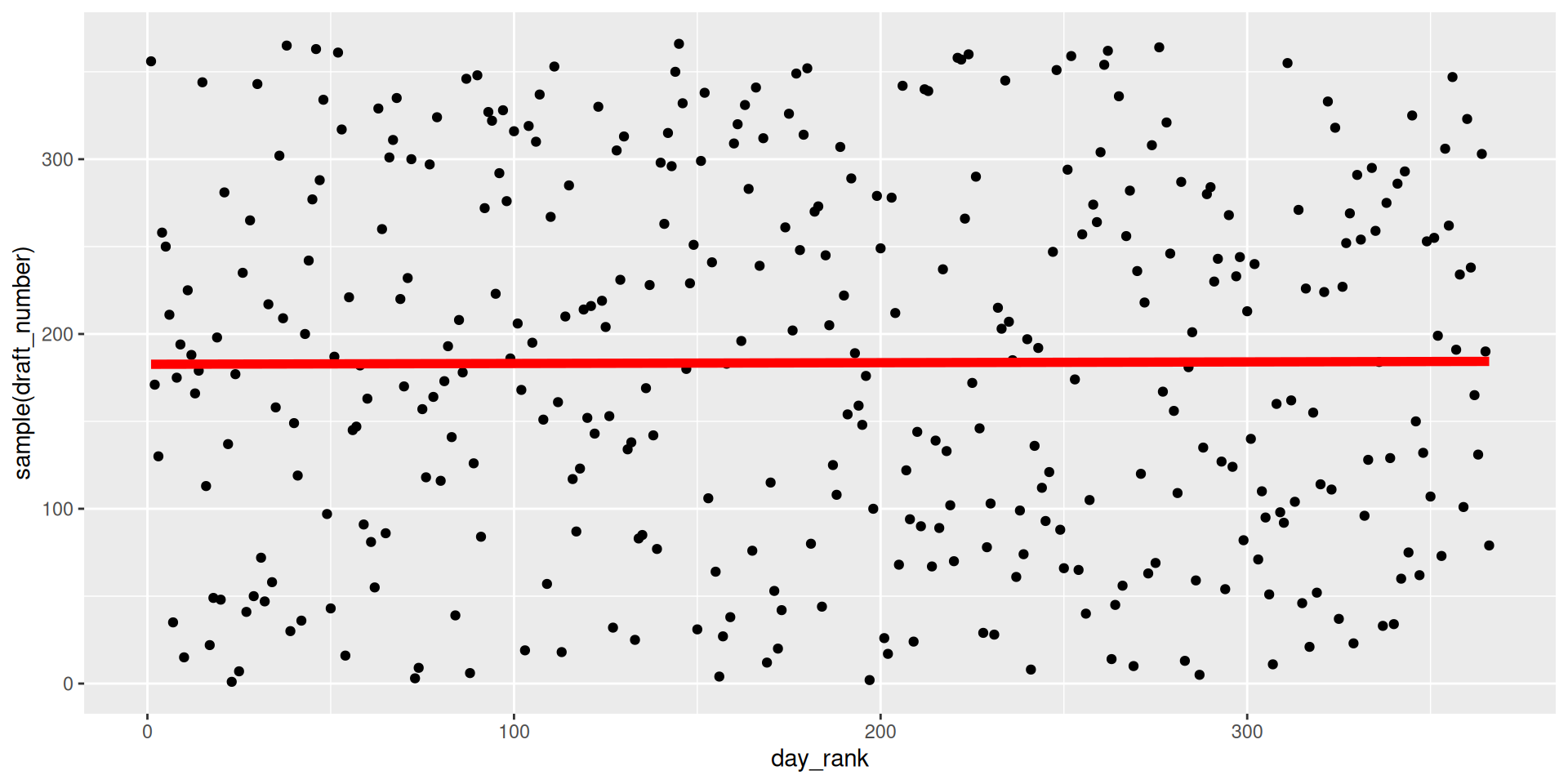
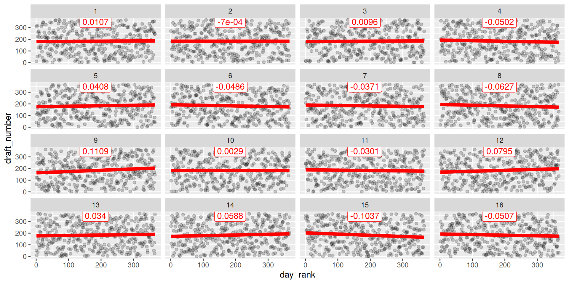
What if we repeat the Vietnam War draft over and over again, randomly scrambling the assignment of draft numbers (\(Y_i\)) to birthdates (\(x_i\))?
Fair draft one
16 more fair drafts
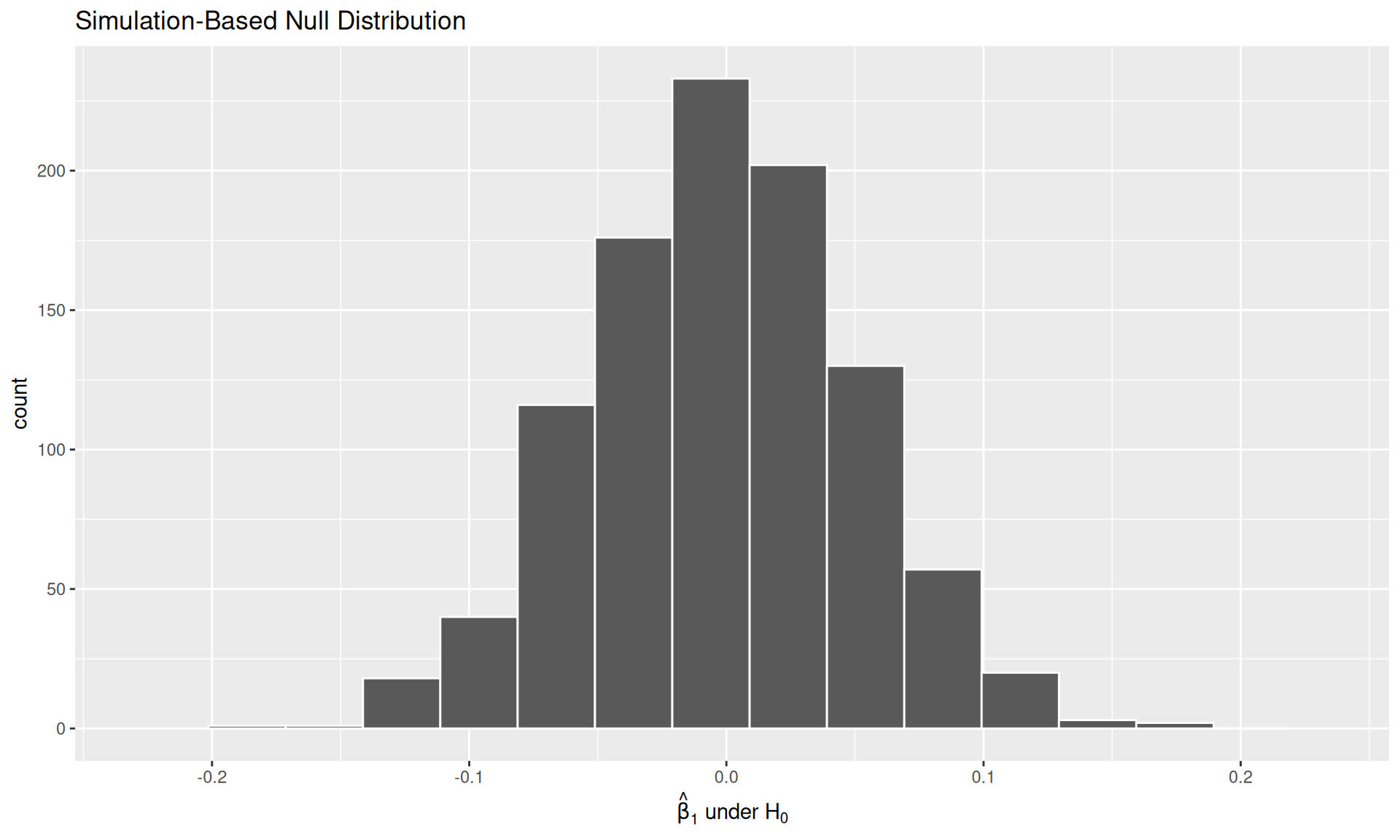
Visualizing the null distribution
All of these fitted slopes under \(H_0\) at once:
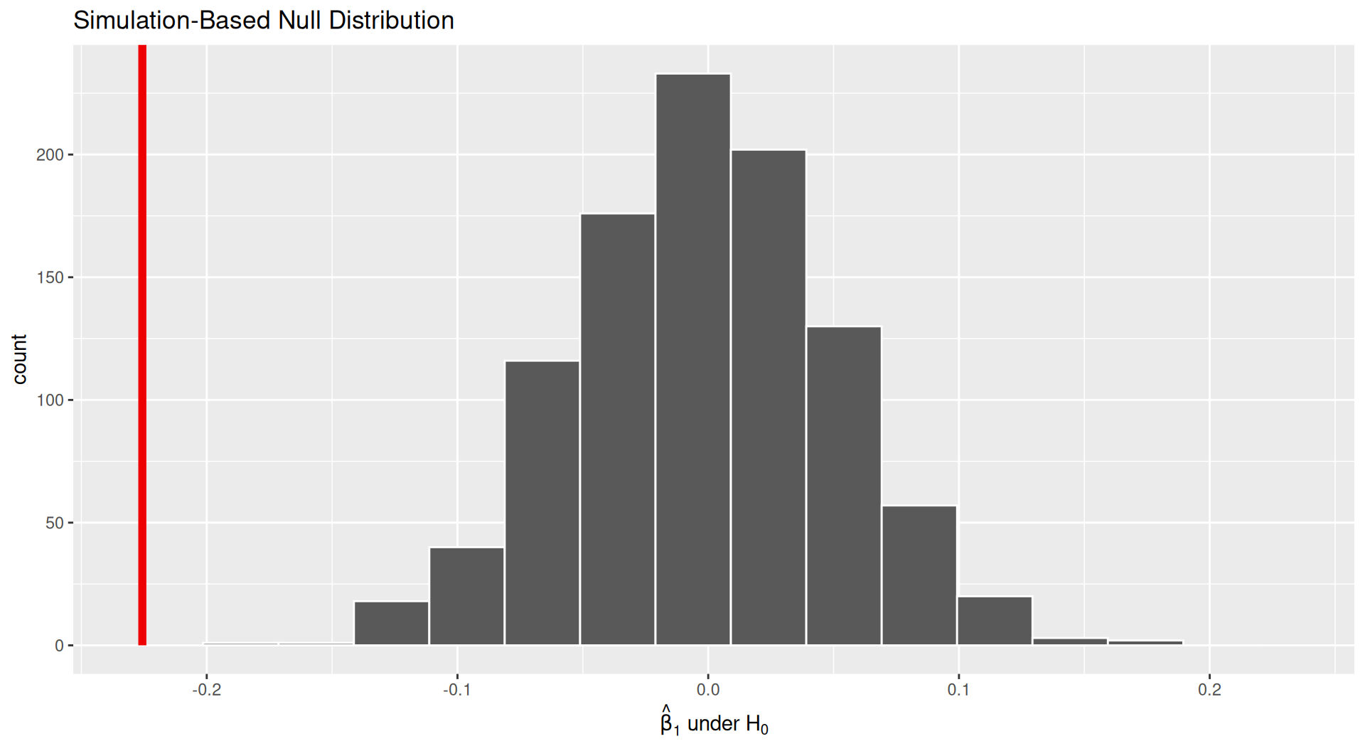
Step 4: Compare the test statistic to the null distribution
What do you notice?
Does \(\widehat{\beta}_1 = -0.226\) fit in?
Step 5: Draw a conclusion in context
Under our null hypothesis…
“A slope like \(\widehat{\beta}_1 = -0.226\) should almost never, ever happen when we conduct a fair draft”
But we observed \(\widehat{\beta}_1 = -0.226\). So either:
- We got incredibly “lucky” and saw a highly unusual outcome
- Our original assumption (the null hypothesis) was wrong
Note
We reject the null hypothesis and conclude that the Vietnam War Draft of 1969 was not a fair draft (\(p < 0.001\)).
What if the evidence wasn’t as clear?
We use the \(p\)-value in conjunction with a decision rule!
- \(p\)-value summarizes the strength of the evidence against \(H_0\)
- Smaller \(p\)-values \(\iff\) more evidence
- A “small enough” \(p\)-value tells us there is a statistically significant difference
- “Small enough” determined by the \(\alpha\)-level
- Typically choose \(\alpha = 0.05\) or \(\alpha = 0.1\)
- Does not mean that this difference is practically important

SDS 291