04-Inference via Probability Distributions
SDS 291
September 17, 2025
Recall: permutation test
Hypothesis testing
Step 1: Formulate null hypothesis
Step 2: Calculate test statistic
Response: draft_number (numeric)
Explanatory: day_rank (numeric)
# A tibble: 1 × 1
    stat
   <dbl>
1 -0.226
Step 3: Generate null distribution
Response: draft_number (numeric)
Explanatory: day_rank (numeric)
Null Hypothe...
# A tibble: 6 × 2
  replicate     stat
      <int>    <dbl>
1         1 -0.0237
2         2 -0.0140
3         3 -0.0153
4         4 -0.0275
5         5  0.00467
6         6  0.0811
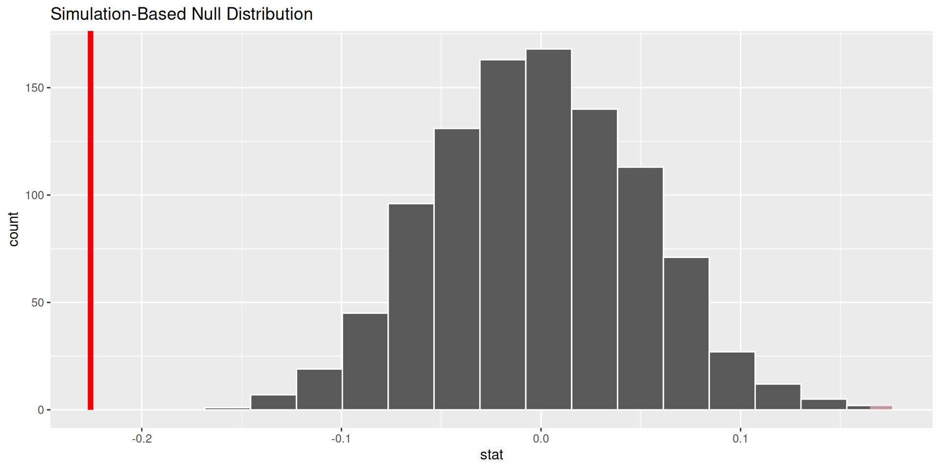
Step 4: Situate the test statistic
Step 5: Draw conclusion
Note
We reject the null hypothesis and conclude that the Vietnam War Draft of 1969 was not a fair draft (\(p < 0.001\)).
What if we didn’t have a computer?
Cobb (2007): A Ptolemaic Curriculum?
I argue that despite broad acceptance and rapid growth in enrollments, the consensus curriculum is still an unwitting prisoner of history. What we teach is largely the technical machinery of numerical approximations based on the normal distribution and its many subsidiary cogs. This machinery was once necessary, because the conceptually simpler alternative based on permutations was computationally beyond our reach. Before computers statisticians had no choice. These days we have no excuse. Randomization-based inference makes a direct connection between data production and the logic of inference that deserves to be at the core of every introductory course.
Inference via probability distribution?
- Steps 1, 2, 4, 5 are the same!
- Problem: don’t have computer to generate the null distribution in Step 3
Solution
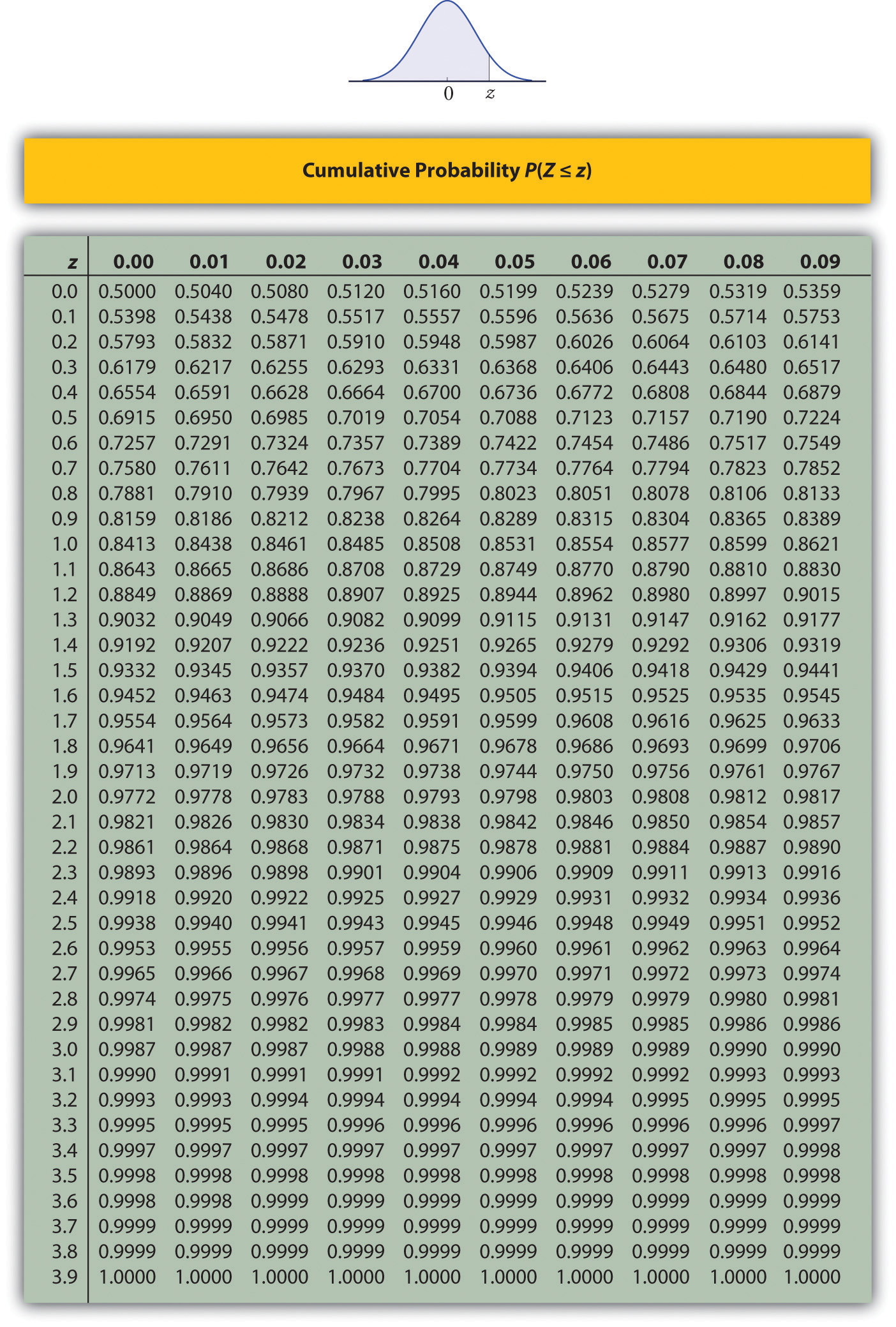
- Statisticians used probability theory to derive parametric distributions for many test statistics in many situations (including the slope coefficient in a linear regression model)!
- Irony: still can’t compute most of them by hand, have to use tables in the back of the book!
Statisticians have shown that
Simple Linear Regression Model
\[ Y_i = \beta_0 + \beta_1 x_i + \epsilon_i, \quad\text{where } \epsilon_i \overset{iid}{\sim} N(0, \sigma_\epsilon) \]
If conditions (TBD) are met (because math):
- Test statistic: \(T = \frac{\widehat{\beta}_1}{\widehat{SE}_{\widehat{\beta}_1}}\)
- \(T\) has a sampling distribution (in this case, a null distribution)
- That sampling distribution is a \(t\)-distribution with \(n-2\) degrees of freedom
In R
Call:
lm(formula = draft_number ~ day_rank, data = draft_data)

Residuals:
     Min       1Q   Median       3Q      Max
-210.758  -85.618   -1.756   84.612  196.150

Coefficients:
             Estimate Std. Error t value Pr(>|t|)
(Intercept) 224.91341   10.81202   20.80  < 2e-16 ***
day_rank     -0.22569    0.05106   -4.42 1.31e-05 ***
---
Signif. codes:  0 '***' 0.001 '**' 0.01 '*' 0.05 '.' 0.1 ' ' 1

Residual standard error: 103.2 on 364 degrees of freedom
Multiple R-squared:  0.05093,   Adjusted R-squared:  0.04833
F-statistic: 19.54 on 1 and 364 DF,  p-value: 1.305e-05
Where does \(T\) come from?
- Recall: \(Z\)-scores
- \(\widehat{\beta}_1\) is the observed slope
- 0 is the hypothesized slope
- \(\widehat{SE}_{\widehat{\beta}_1}\) is the standard error of the slope coefficient
- \(T\) is kind of like a \(Z\)-score, but different
- \(T \sim t(n-2)\)
Tip
The standard error is just the standard deviation of the sampling distribution!
What is the standard error (of the slope)?
\[\begin{align*} \widehat{SE}_{\widehat{\beta}_1} &= \frac{1}{\sqrt{n-1}} \cdot \frac{\hat{\sigma}_\epsilon}{\hat{\sigma}_X} \\ &= \frac{1}{\sqrt{n-1}} \cdot \frac{\hat{\sigma}_\epsilon}{s_X} \\ &= \frac{1}{\sqrt{n-1}} \cdot \frac{\text{st. dev. of errors}}{\text{st. dev. of }X} \end{align*}\]
What is the standard error (of the model)?
\[\begin{align*} \widehat{\sigma}_\epsilon &= \sqrt{\frac{SSE}{n-2}} \\ &= \sqrt{\frac{1}{n-2}\sum_{i=1}^{n}e_i^2} \\ &= \sqrt{\frac{1}{n-2}\sum_{i=1}^{n}(y_i - \widehat{y}_i)^2} \end{align*}\]
What is the t-distribution?

Write them all down
Call:
lm(formula = draft_number ~ day_rank, data = draft_data)

Residuals:
     Min       1Q   Median       3Q      Max
-210.758  -85.618   -1.756   84.612  196.150

Coefficients:
             Estimate Std. Error t value Pr(>|t|)
(Intercept) 224.91341   10.81202   20.80  < 2e-16 ***
day_rank     -0.22569    0.05106   -4.42 1.31e-05 ***
---
Signif. codes:  0 '***' 0.001 '**' 0.01 '*' 0.05 '.' 0.1 ' ' 1

Residual standard error: 103.2 on 364 degrees of freedom
Multiple R-squared:  0.05093,   Adjusted R-squared:  0.04833
F-statistic: 19.54 on 1 and 364 DF,  p-value: 1.305e-05
Sampling distribution of \(\widehat{\beta}_0\)
Normal, with:
\[ \widehat{\beta}_0 \sim N \left( \beta_0, \underbrace{ \sigma_\epsilon \sqrt{\frac{1}{n} + \frac{\bar{x}^2}{(n-1)s_x^2}}}_{SE(\widehat{\beta}_0)} \right) \]
Sampling distribution of \(\widehat{\beta}_1\)
Normal, with:
\[ \widehat{\beta}_1 \sim N \left( \beta_1, \underbrace{ \sigma_\epsilon \sqrt{\frac{1}{(n-1)s_x^2}}}_{SE(\widehat{\beta}_1)} \right) \]
Disentangling variability
- Variance and standard deviation are two different measures of spread
- Variance: \(Var(Y) = \sigma^2\)
- Standard deviation: \(SD(Y) = \sqrt{Var(Y)} = \sigma\)
- If the distribution we are characterizing is a sampling distribution:
- Call the standard deviation the standard error: \(SE(Y)\)
Don’t confuse:
- Spread of the error terms, \(\epsilon\)
- Captured by: standard deviation, \(SD(\epsilon) = \sigma_\epsilon\)
- Tells us about: amount of noise in the data \(\iff\) spread of the responses about the population regression model
- Estimated by: \(\widehat{\sigma}_\epsilon\)
- Spread of the sampling distribution for \(\widehat{\beta}_0\) and \(\widehat{\beta}_1\)
- Captured by: standard errors, \(SE_{\widehat{\beta}_0}\) and \(SE_{\widehat{\beta}_1}\)
- Tells us about: sampling variability \(\iff\) how the estimated intercepts and slopes differ from sample to sample
- Estimated by: \(\widehat{SE}_{\widehat{\beta}_1}, \widehat{SE}_{\widehat{\beta}_0}\)
Conditions
Conditions on the random error
Simple Linear Regression Model
\[Y_i = \beta_0 + \beta_1 x_i + \epsilon_i, \quad\text{where } \epsilon_i \overset{iid}{\sim} N(0, \sigma_\epsilon)\]
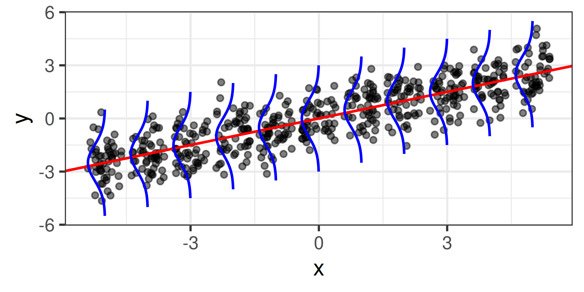
- True model for expected value of \(Y_i\) in terms of \(x_i\) is a line: \[E[Y_i|x_i] = \beta_0 + \beta_1x_i\]
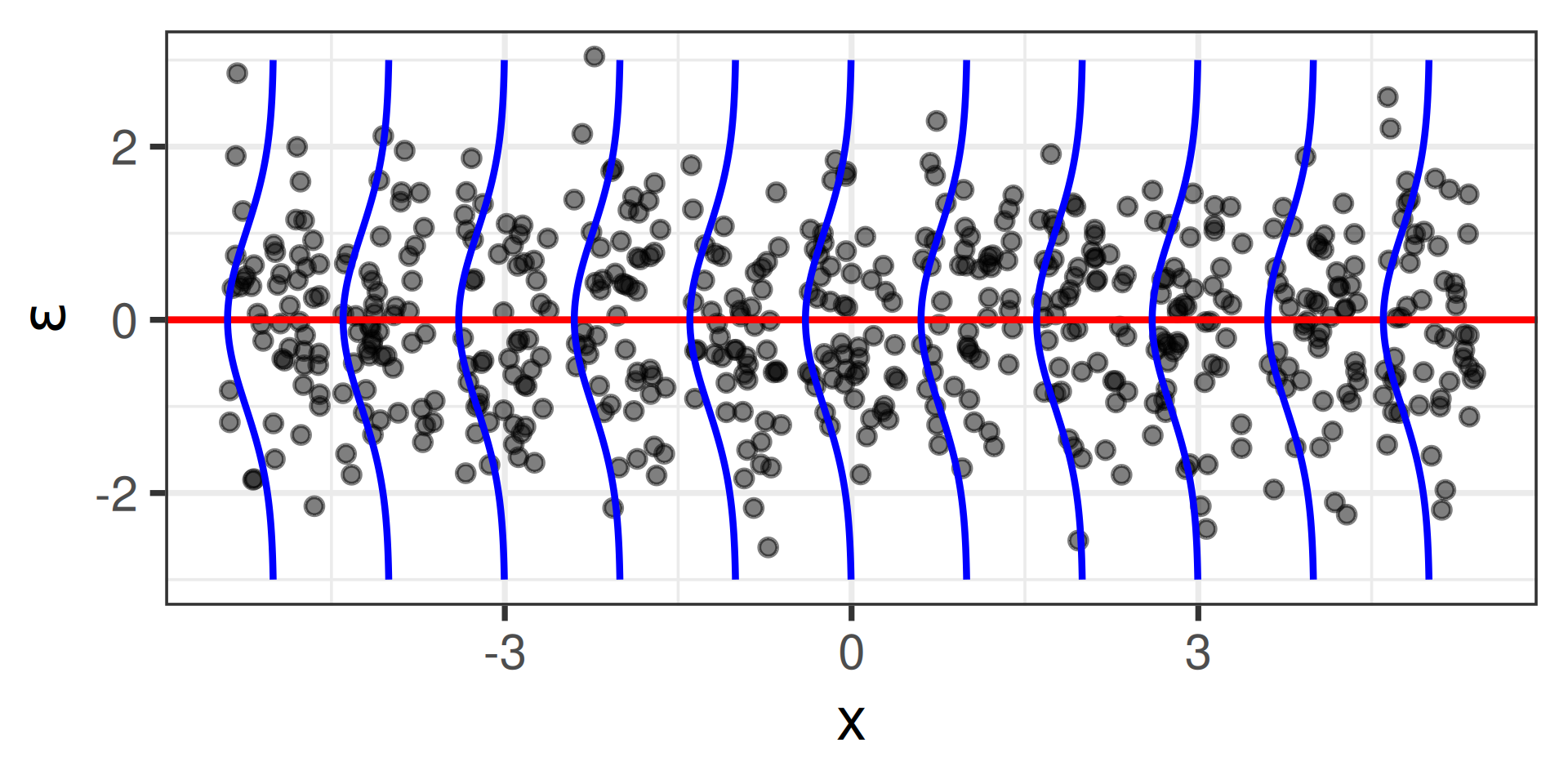
- Errors are independent and identically distributed (iid)
- Errors follow a Normal distribution
- Errors have mean zero (for all values of \(x_i\))
- Variance of the errors, \(\sigma_\epsilon^2\), are equal (for all values of \(x_i\))
Visualizing the conditions
In terms of response variable \(Y_i\)
In terms of errors \(\epsilon_i = Y_i - E[Y_i | x_i]\)
The \(t\)-test
Hypothesis testing for the slope
Note
Does a (linear) relationship exist between the explanatory variable and the response variable?
- Formulate hypotheses: \(H_0: \beta_1 = 0\) vs. \(H_A: \beta_1 \neq 0\)
- Compute test statistic: \[T = \frac{\text{estimate} - \text{hypothesized value}}{\text{estimated standard error}} = \frac{\widehat{\beta}_1 - 0}{\widehat{SE}_{\widehat{\beta}_1}}\]
- Generate null distribution: \(t_{n-2}\)
In context
Note
Does a (linear) relationship exist between birth date and draft number? In other words, was the Vietnam War draft process in 1969 fair?
               Estimate  Std. Error   t value     Pr(>|t|)
(Intercept) 224.9134067 10.81202040 20.802163 6.830736e-64
day_rank     -0.2256861  0.05106196 -4.419849 1.305208e-05
Calculate test statistic: \[T = \frac{\widehat{\beta}_1 - 0}{\widehat{SE}_{\widehat{\beta}_1}} = \frac{-0.226 - 0}{0.051} \approx -4.42\]
Generate the null distribution: \(t_{n-2} = t_{366 - 2}\)
Situate the test statistic
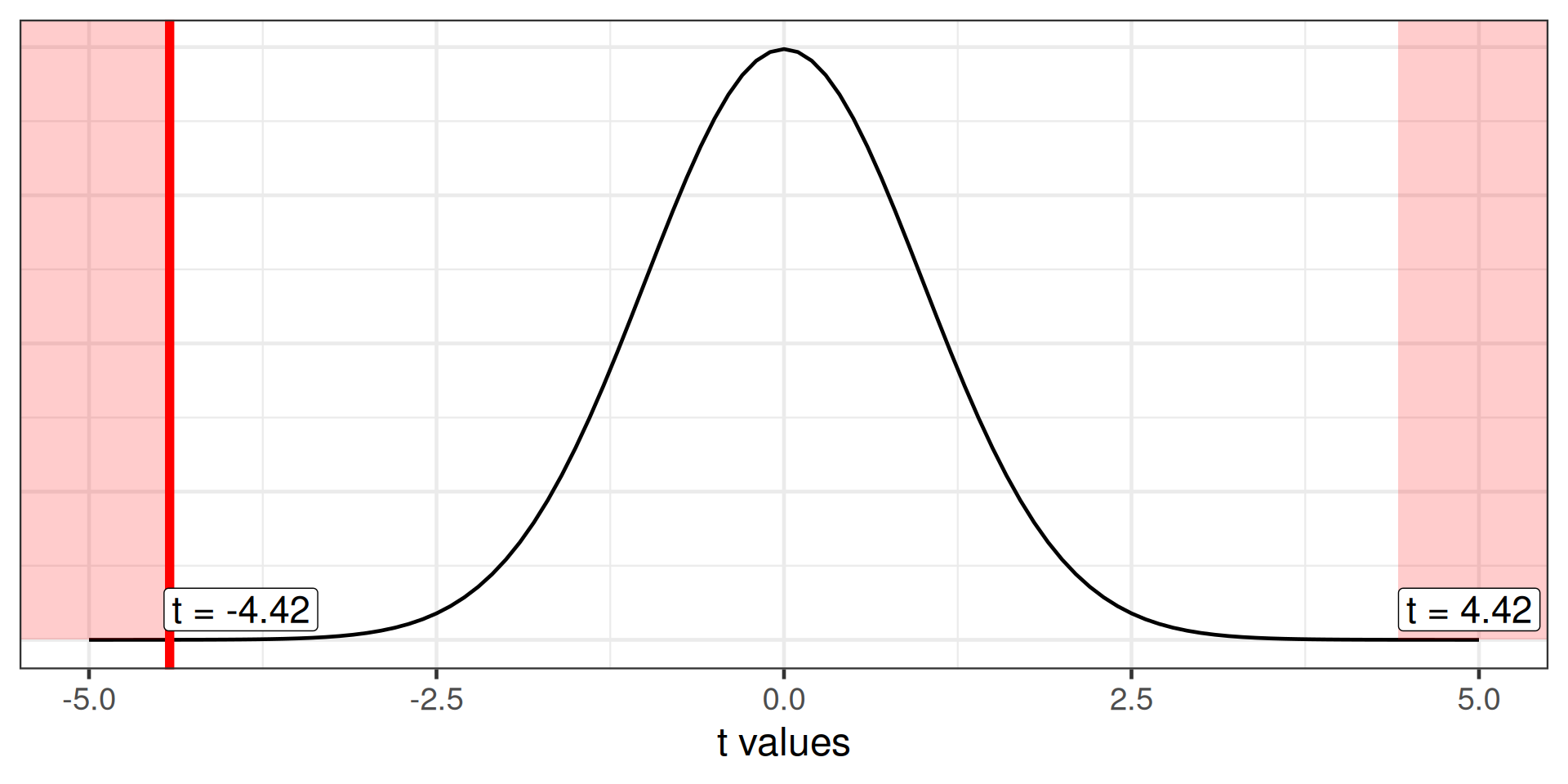
Calculating the p-value
Same conclusion as permutation test!
During the 1969 Vietnam War draft, birth days later in the calendar year were more likely to receive low draft numbers than those earlier in the calendar year: each additional day after January 1 was associated with a draft number that was 0.226 lower, on average, than the day before.
This relationship is statistically significant at the \(\alpha = 0.05\) level, suggesting that the 1969 lottery was not a fair process (\(p < 0.001\)).

SDS 291