05-Confidence Intervals
SDS 291
Prof. Baumer
September 22, 2025
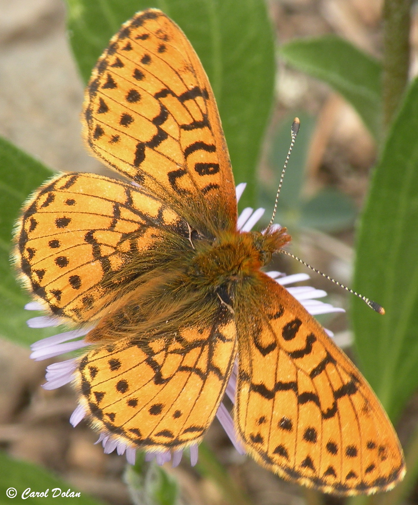
Butterflies
The butterfly effect
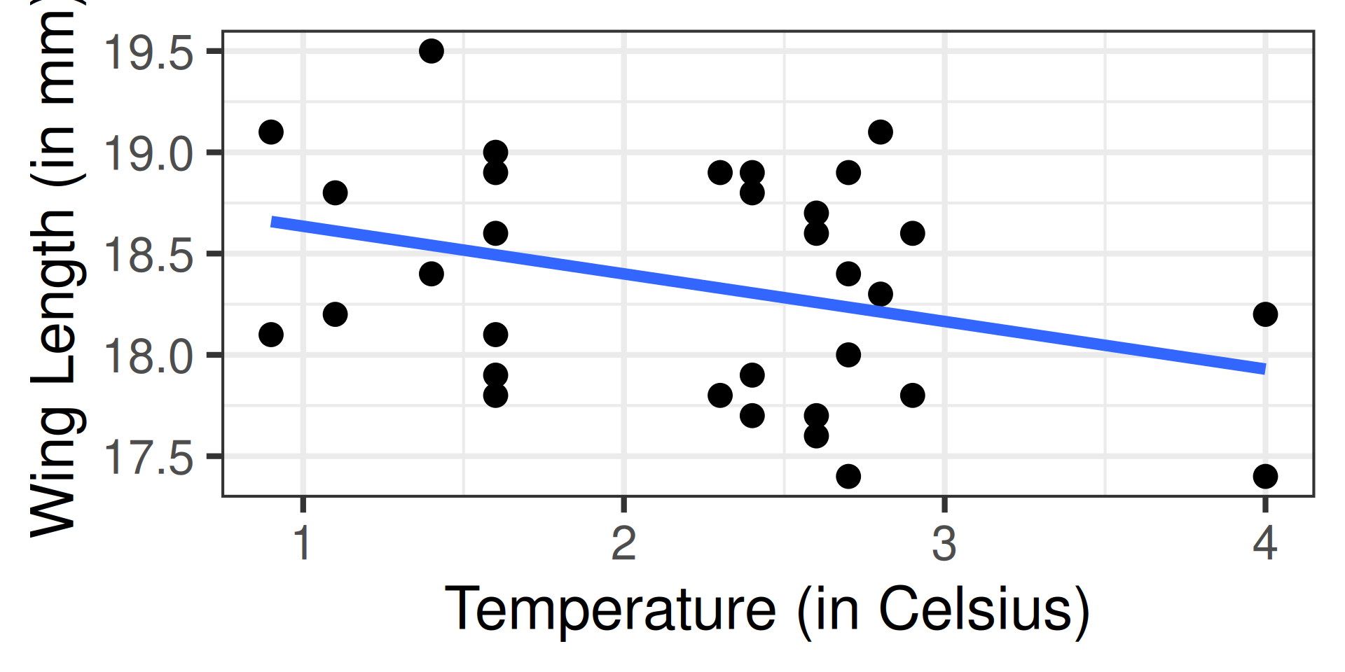
Between 1996 and 2013, scientists sampled 32 Boloria chariclea butterflies and measured their wing length (in mm) and the average temperature (in Celsius) of the preceding summer:
Visualizing butterfly relationships
Note
Your turn! (Exercise 1) What can we say about the relationship between summer temperatures and butterfly wing length?
Confidence Intervals
Review: what is a confidence interval?
- Point estimate: What is our best guess for the unknown true value of the slope, \(\beta_1\)?
- Hypothesis test: Is the true value of the slope equal to 0?
- Confidence interval: What is a range of “plausible values” for the true slope?
Fishing analogy

Review: what is a confidence interval?
\[ \text{point estimate } \pm \underbrace{q^* \cdot \widehat{SE}}_{\text{margin of error}} \] where:
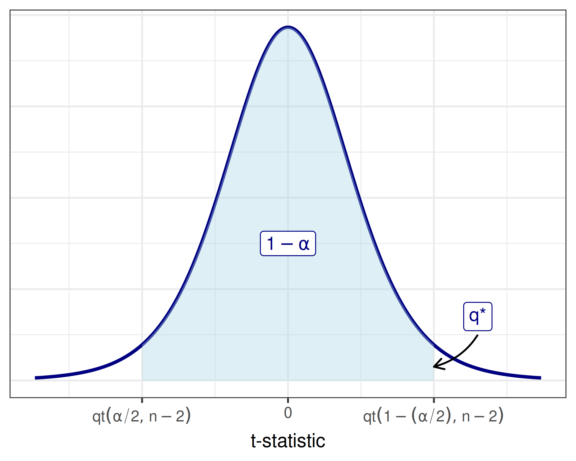
- \(q^*\): a critical value that captures information about the confidence level of the interval
- \(\widehat{SE}\): the estimated standard error of the point estimate
Review: the confidence level is \((1 - \alpha) 100\%\) means
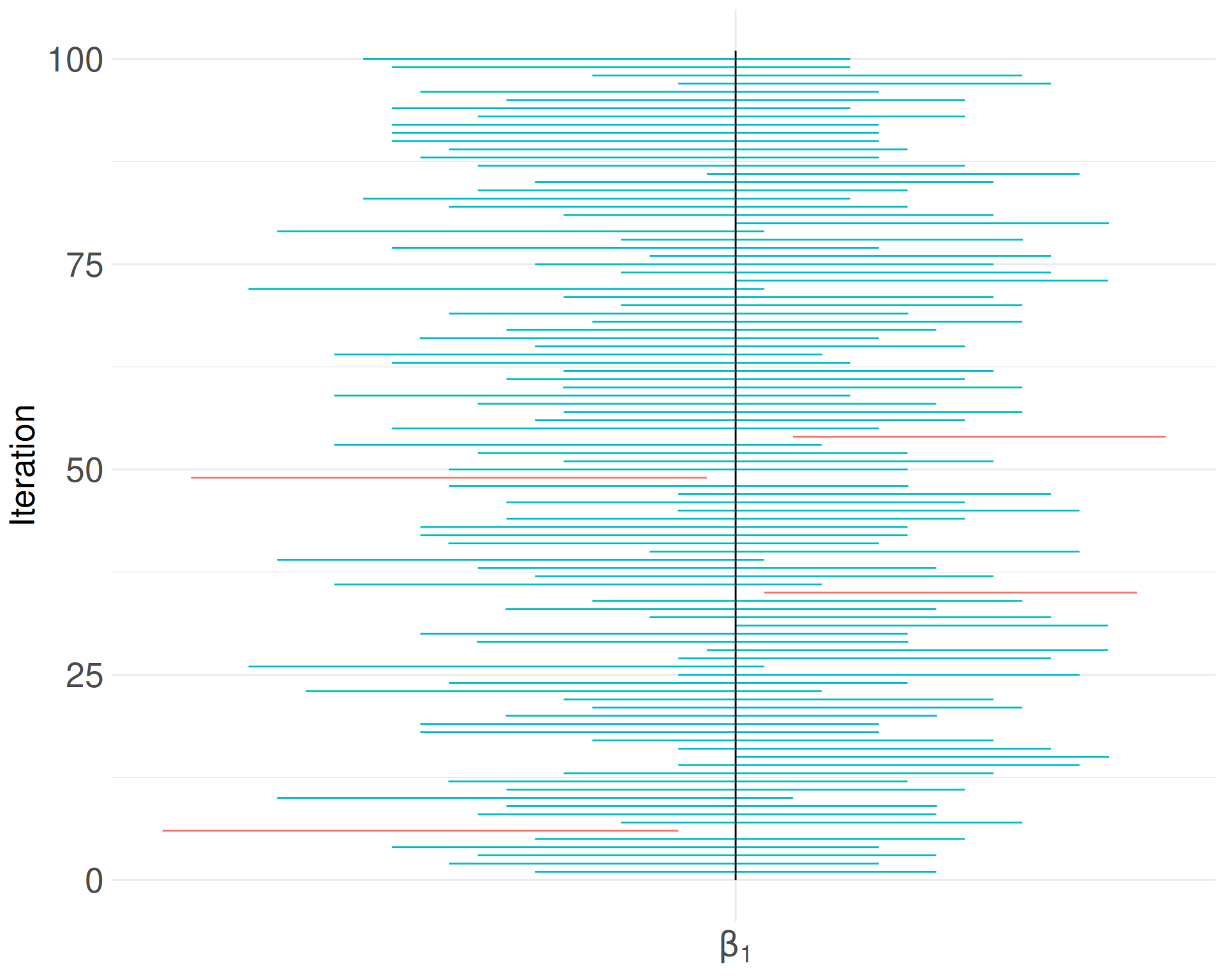
- If we repeated the process of taking a sample, finding the point estimate, and adding and subtracting the margin of error over and over again, then \((1-\alpha) 100\)% of the intervals would capture the truth
Review: the confidence level is \((1 - \alpha) 100\%\) means
- Our interval contains all of the plausible values \(\beta^*\) that we would not have rejected with a two-sided, level \(\alpha\) test of \(H_0: \beta_1 = \beta^*\)
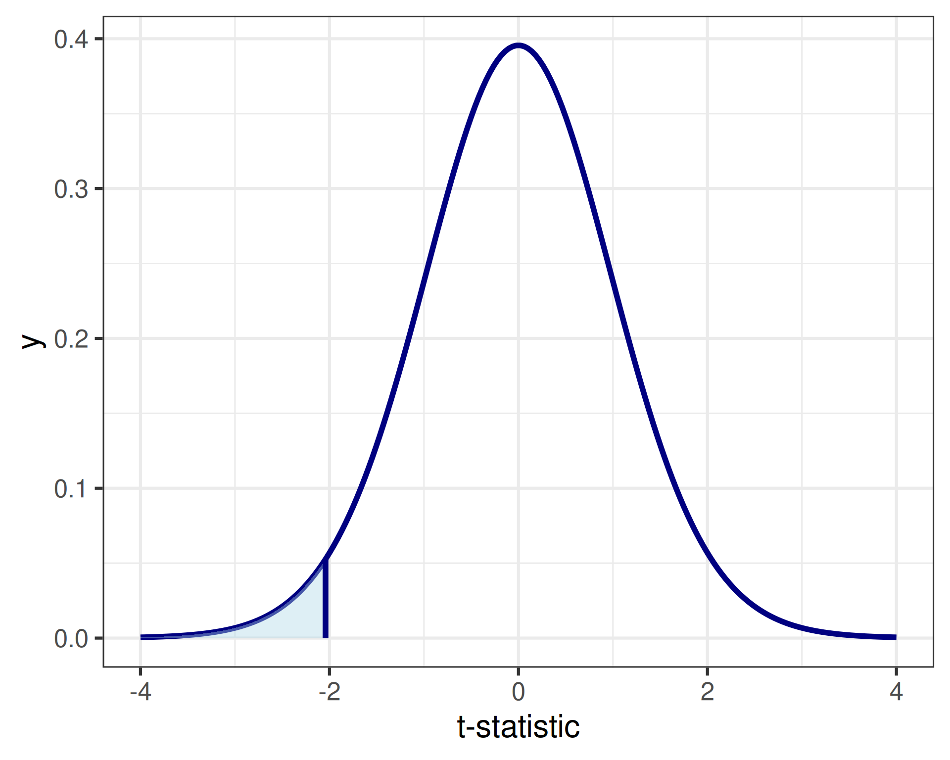
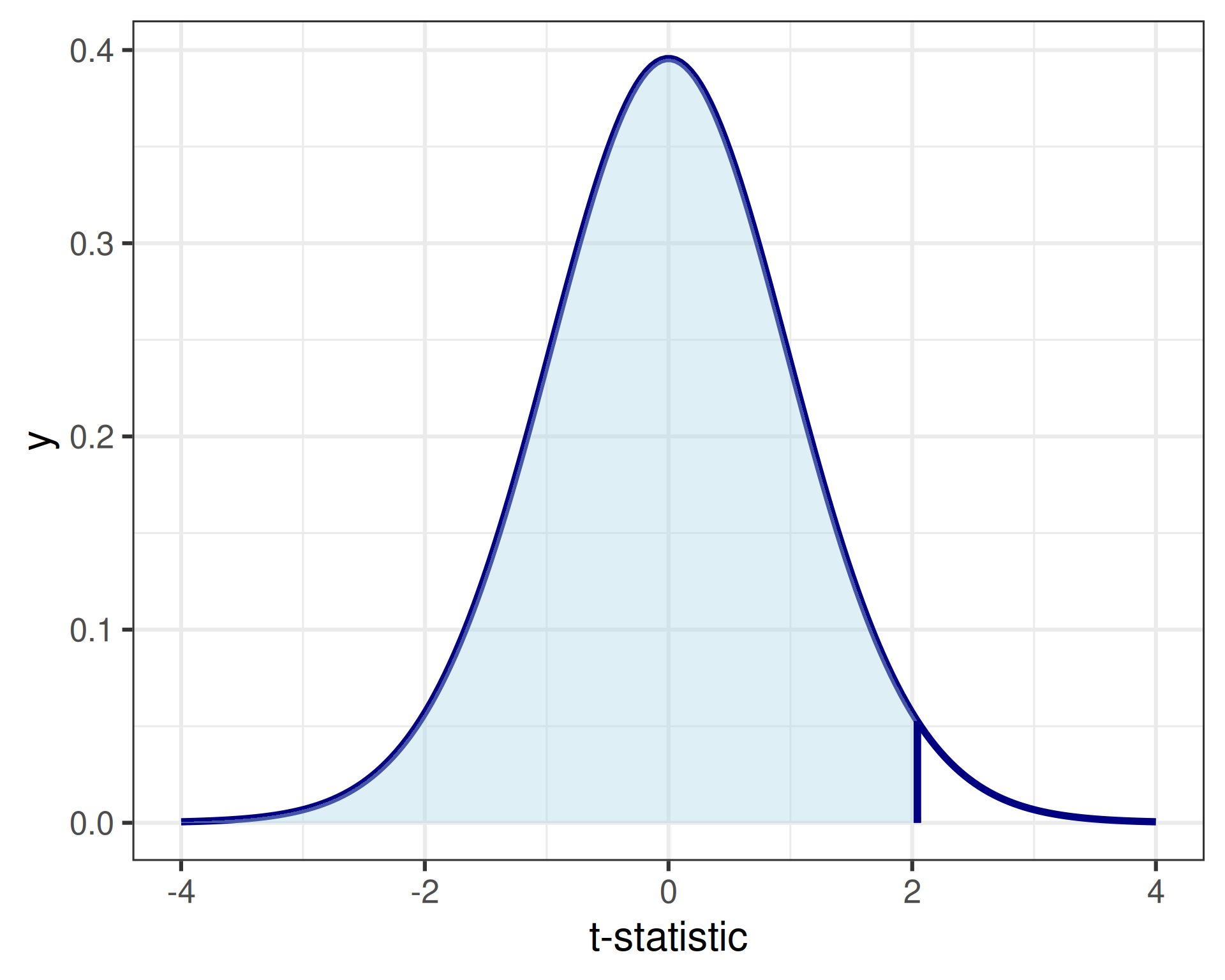
Aside: quantiles
Butterfly Example: 95% Confidence Interval
Confidence Interval for the Slope
\[ \widehat{\beta}_1 \pm t^*\times \widehat{SE}(\widehat{\beta}_1), \] where \(t^*\) is the \(1 - (\frac{\alpha}{2})\) percentile of a \(t_{n-2}\) distribution
              Estimate Std. Error   t value     Pr(>|t|)
(Intercept) 18.8698426  0.2870393 65.739581 5.471606e-34
Temp -0.2350416 0.1218277 -1.929296 6.320053e-02\[ -0.235 \pm (2.04)(0.122) = (-0.484,\ 0.014) \]
Alternatively
                 2.5 %      97.5 %
(Intercept) 18.2836302 19.45605505
Temp -0.4838469 0.01376368Confidence intervals for the slope
Interpretation:
Tip
We are confidence level confident that a one unit increase in the explanatory variable is associated with between a lower bound [increase/ decrease] and an upper bound [increase/decrease] in the average value of the response variable.
Butterfly Example: 95% Confidence Interval
Tip
We are 95% confident that a one degree Celsius increase in the average summer temperature is associated with between a 0.484 mm decrease and a 0.014 mm increase in the average length of Boloria chariclea wings.
Types of intervals
| Representative Research Question | Target of Inference | Interval |
|---|---|---|
| What is the relationship between summer temperatures and the length of Boloria chariclea wings? | True Slope, \(\beta_1\) | CI for a slope |
| What is the mean wing length across all Boloria chariclea butterflies after a summer with an average temperature of 2°C? | Subpopulation mean, \(\mu(x^*)\) | CI for a mean |
| What is the wing length of one Boloria chariclea butterfly exposed to those conditions? | Individual response, \(y_\text{new}(x^*)\) | PI for an individual |
Prediction intervals
Your turn!
Turn to Exercise 2 on the handout!
Spend about two minutes (on your own) considering what type of interval is most appropriate for each of the four scenarios.
After the two minutes is up, discuss your answers with your neighbor!
Obtaining point estimates
Estimated Mean Wing Length When Summer Temps are \(2^\circ\)C:
\[ \widehat{\mu}(2) \equiv \widehat{y} = 18.870 - 0.234\left(2\right) = 18.4\text{ mm} \]
Predicted Wing Length for an Individual Butterfly with \(x = 2^\circ\)C:
\[ \widehat{y}_\text{new}(2) \equiv \widehat{y} = 18.870 - 0.234\left(2\right) = 18.4\text{ mm} \]
SE for mean: \(\widehat{\mu}(x^*)\)
- Captures the spread in the estimated value of the mean response across multiple samples from the population
- If we took repeated samples of \(n = 32\) butterflies, how much would we expect our estimated mean wing length at \(x^* = 2^\circ\)C to differ from sample to sample?
\[ \widehat{SE} \left( \widehat{\mu}(x^*)\right) = \widehat{\sigma}\sqrt{\frac{1}{n} + \frac{(x^* - \bar{x})^2}{(n-1)s_x^2}} \]
- \(\bar{x}\): average of the explanatory variable
- \(s_x^2\): sample variance of the explanatory variable
- \(\widehat{\sigma_\epsilon}\): the estimated standard deviation of the error term
SE for predicted value: \(\widehat{y}_\text{new}(x^*)\)
- Spread in the individual new observations with \(x = x^*\)
- How much variability do we see in the wing lengths of individual butterflies exposed to average summer temperatures of \(x^* = 2^\circ\)C?
\[\begin{align*} \widehat{SE} \left( \widehat{y}_\text{new}(x^*) \right) &= \widehat{\sigma}\sqrt{1 + \frac{1}{n} + \frac{(x^* - \bar{x})^2}{(n-1)s_x^2}} \\ &= \sqrt{{\widehat{\sigma}^2} + {\widehat{SE} \left( \widehat{\mu}(x^*) \right)^2}} \end{align*}\]
Building CI for the mean
- CI for the mean response at a particular \(x^*\): \[ \widehat{\mu}(x^*) \pm t^* \cdot \widehat{SE} \left( \widehat{\mu}(x^*) \right) \] \((1-\alpha) 100\)% of intervals constructed this way (across repeated samples) will include the true mean response in the subpopulation with \(x = x^*\)
Building a PI for an observation
- PI for an individual response at a particular \(x^*\) \[ \widehat{y}_\text{new}(x^*) \pm t^* \cdot \widehat{SE} \left( \widehat{y}_\text{new}(x^*) \right) \] \((1-\alpha) 100\)% of intervals constructed this way (across repeated samples) will include the future value of the response when \(x = x^*\)
Using augment()
augment()from broom package 🧹.fitted: the fitted value, \(\widehat{y}_i\).resid: the corresponding residual, \(e_i\)
# A tibble: 32 × 8
    Wing  Temp .fitted  .resid   .hat .sigma  .cooksd .std.resid
   <dbl> <dbl>   <dbl>   <dbl>  <dbl>  <dbl>    <dbl>      <dbl>
 1  18.1   0.9    18.7 -0.558  0.123   0.532 0.0870       -1.12
 2  18.2   1.1    18.6 -0.411  0.0971  0.537 0.0353       -0.810
 3  18.4   1.4    18.5 -0.141  0.0667  0.543 0.00266      -0.273
 4  18.1   1.6    18.5 -0.394  0.0516  0.538 0.0156       -0.757
 5  17.9   1.6    18.5 -0.594  0.0516  0.531 0.0354       -1.14
 6  17.8   1.6    18.5 -0.694  0.0516  0.527 0.0484       -1.33
 7  17.8   2.3    18.3 -0.529  0.0315  0.534 0.0165       -1.01
 8  17.9   2.4    18.3 -0.406  0.0328  0.538 0.0101       -0.772
 9  17.7   2.4    18.3 -0.606  0.0328  0.531 0.0226       -1.15
10  18.3   2.8    18.2  0.0883 0.0485  0.543 0.000731      0.169
# ℹ 22 more rows
Confidence intervals with augment()
newdataargument: a new data set with:- same vars as explanatory variables in model
- value(s) \(x^*\) that we are interested in
Predictions intervals with augment()
Interpretation
CI for the mean response
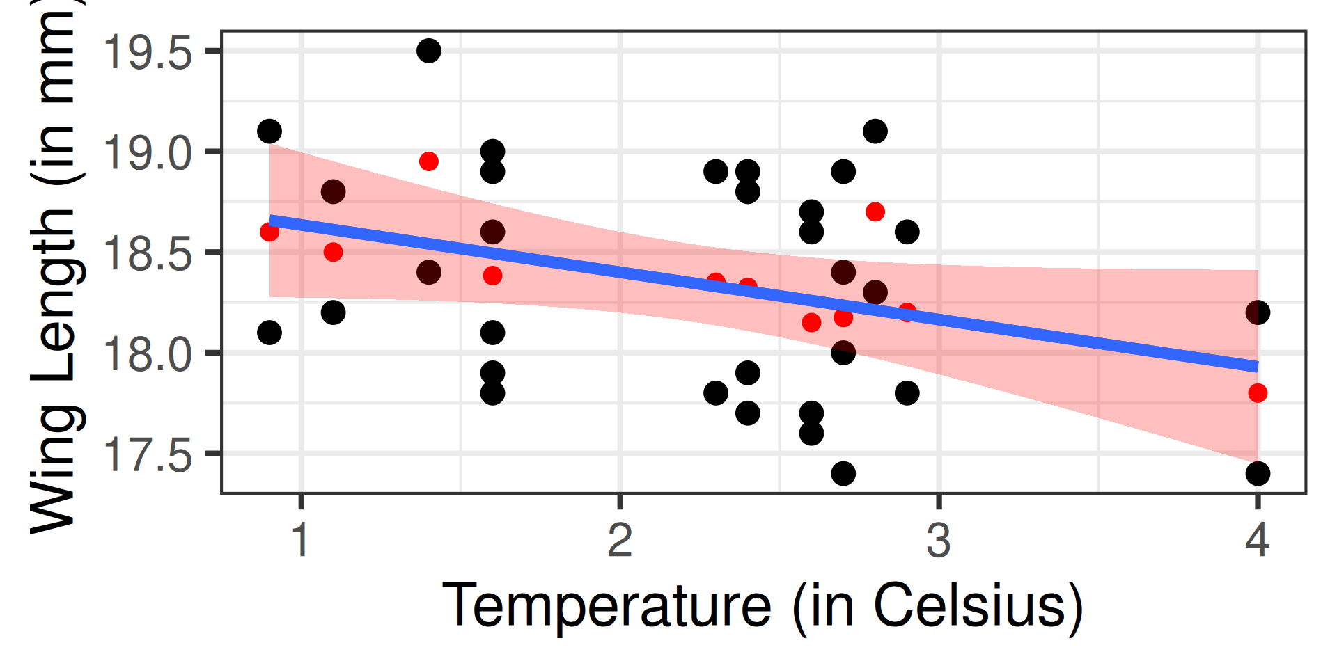
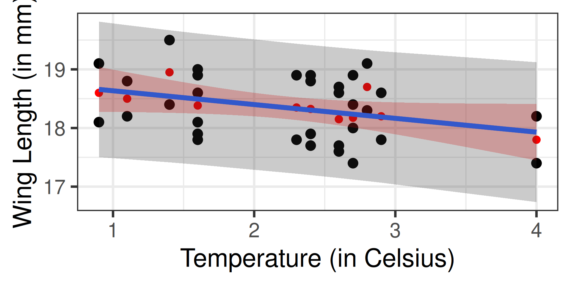
We are 95% confident that the true mean wing length among the subpopulation of Boloria chariclea butterflies found following a summer with an average temperature of 2\(^\circ\)C is between 18.2 mm and 18.6 mm.
PI for an individual response
We are 95% confident that the wing length of an individual Boloria chariclea butterfly found following a summer with an average temperature of 2\(^\circ\)C is between 17.3 mm and 19.5 mm.
Adding CIs to a plot
CIs on a plot
Adding PIs to a plot
Visualizing the intervals

SDS 291