07-Transformations

SDS 291

Prof. Baumer

September 29, 2025

Movies in 2008

Example: Quantum of Solace

Research Question

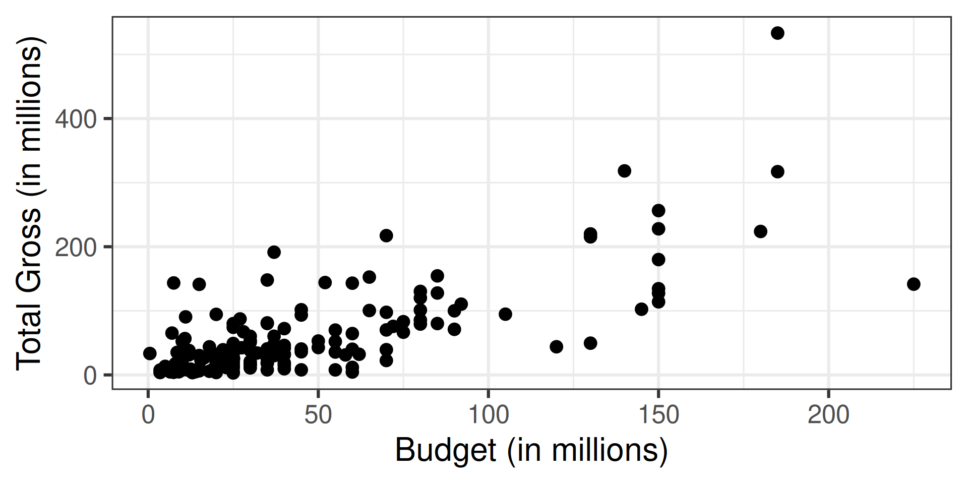
As newly-minted movie executives at Columbia Pictures circa 2008, we’d like to know whether our $200,000,000 investment in the movie Quantum of Solace will pay off.

  • Given the size of the movie’s budget, what do we predict its total box office gross to be?

Example: box office revenues in 2008
Checking regression conditions in R

  • Download the movies data:
movies <- read_csv("https://raw.githubusercontent.com/kaitlyncook/data-sets/main/movies-08.csv")
  • Create two new variables for the Budget_2008 and Total_Gross in millions of dollars
  • Fit the regression model
  • Draw diagnostic plots and assess the conditions

Good news 😄

  • Mild violations of the regression conditions are expected: it’s one of the hazards of doing business with real data!
  • Linear regression is generally robust to violations of:
    • Normality
      • Necessary for determining the correct distribution for hypothesis testing and confidence intervals when the sample size is small or our focus is on prediction for a single observation
      • Otherwise, the Central Limit Theorem saves us!

Bad news 🙍

Linear regression is generally less robust to violations of:

  1. Linearity
    • Necessary for our estimated regression coefficients to, on average, give us the correct answer!
  2. Independence
  3. Equal Variance
    • Necessary when quantifying \(SE(\widehat{\beta})\), our degree of (un)certainty in our estimated coefficients!

What should we do if our model does severely violate the conditions?

  1. Use permutation tests
    • don’t require conditions on the random error terms
  2. Add additional explanatory variables to the model…
  3. Re-express variables so that the conditions approximately hold for the transformed variables
  4. Select a different type of regression model (beyond those discussed in SDS 291) to model the data:
    • Time series models
    • hierarchical models for dependent data
    • Weighted regression for non-constant variance
    • Generalized linear models

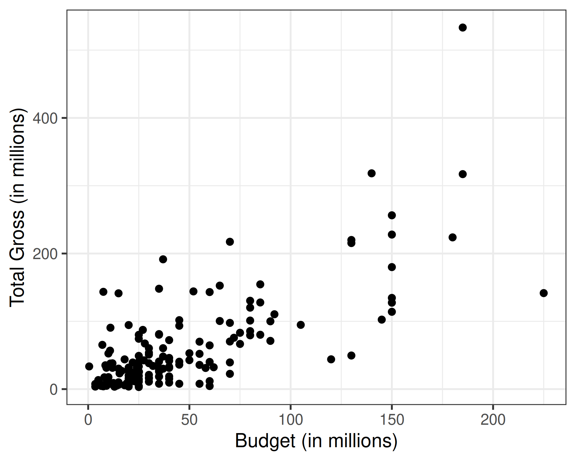
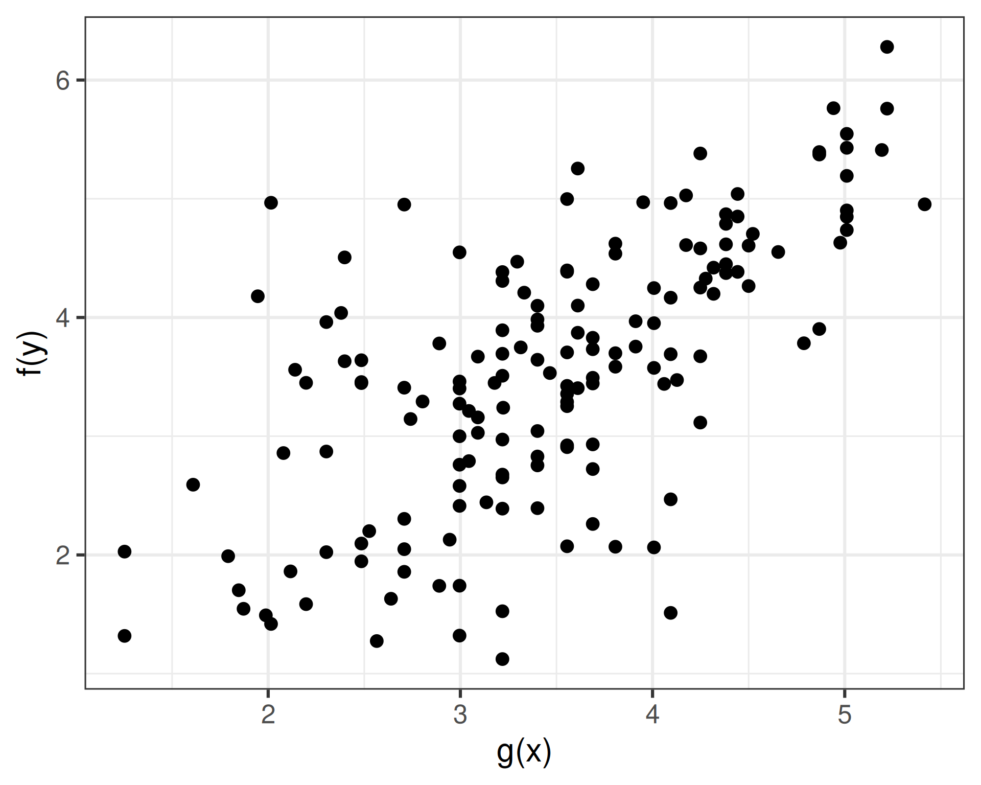
Motivation behind transformations

Is there some function that we can apply to one (or both) of \(x\) and \(Y\) so that the regression conditions seem reasonable for the relationship between the transformed variables?
Selecting a transformation

  • Mostly a trial-and-error process!
  • A few helpful heuristics:
    • Violations of linearity only
      • transform the explanatory variable, \(x\)
      • changes the shape of the relationship!
    • Violations of both linearity and normality or equal variance
      • transform the response variable, \(Y\)
      • changes the error structure (and often the shape, too)!
  • Common transformations: logarithms, reciprocals, square roots, polynomials

Working with transformed models

Hypothesis Testing

  • Transformations/re-expressions won’t create new relationships where there were none previously!
mod_movies_log <- lm(
  log(Total_Gross_M) ~ log(Budget_M),
  data = movies
)
summary(mod_movies_log)

Call:
lm(formula = log(Total_Gross_M) ~ log(Budget_M), data = movies)

Residuals:
    Min      1Q  Median      3Q     Max 
-2.5108 -0.6550  0.1023  0.5687  3.0493 

Coefficients:
              Estimate Std. Error t value Pr(>|t|)    
(Intercept)    0.97649    0.26773   3.647 0.000359 ***
log(Budget_M)  0.74400    0.07487   9.937  < 2e-16 ***
---
Signif. codes:  0 '***' 0.001 '**' 0.01 '*' 0.05 '.' 0.1 ' ' 1

Residual standard error: 0.8933 on 159 degrees of freedom
  (46 observations deleted due to missingness)
Multiple R-squared:  0.3831,    Adjusted R-squared:  0.3792 
F-statistic: 98.75 on 1 and 159 DF,  p-value: < 2.2e-16

Prediction of Individual Response

  • Re-express the prediction back to original data scale
    • apply the inverse transformation
quantum_of_solace <- data.frame(Budget_M = 200)

library(broom)
q_of_s <- mod_movies_log |> 
  augment(newdata = quantum_of_solace, interval = "prediction", conf.level = 0.95)
q_of_s
# A tibble: 1 × 4
  Budget_M .fitted .lower .upper
     <dbl>   <dbl>  <dbl>  <dbl>
1      200    4.92   3.13   6.71
exp(q_of_s)
# A tibble: 1 × 4
  Budget_M .fitted .lower .upper
     <dbl>   <dbl>  <dbl>  <dbl>
1  7.23e86    137.   22.8   820.

Interpretation

Need careful consideration:

  • If the explanatory variable is transformed to \(x' = g(x)\)
    • Does a one unit increase in \(x'\) correspond to a one unit increase in \(x\)?
    • Is a one unit increase the most meaningful kind of change for us to consider when describing the relationship between our two variables?
  • If the response variable has been transformed to \(y' = f(y)\)
    • Does the mean of the transformed response variable correspond in any way to the mean (or another useful summary) of the untransformed response variable?