09-Interpretting Transformations
SDS 291
Prof. Baumer
October 6, 2025
Interpretting Transformed Models
Quantum of Solace
Research Question
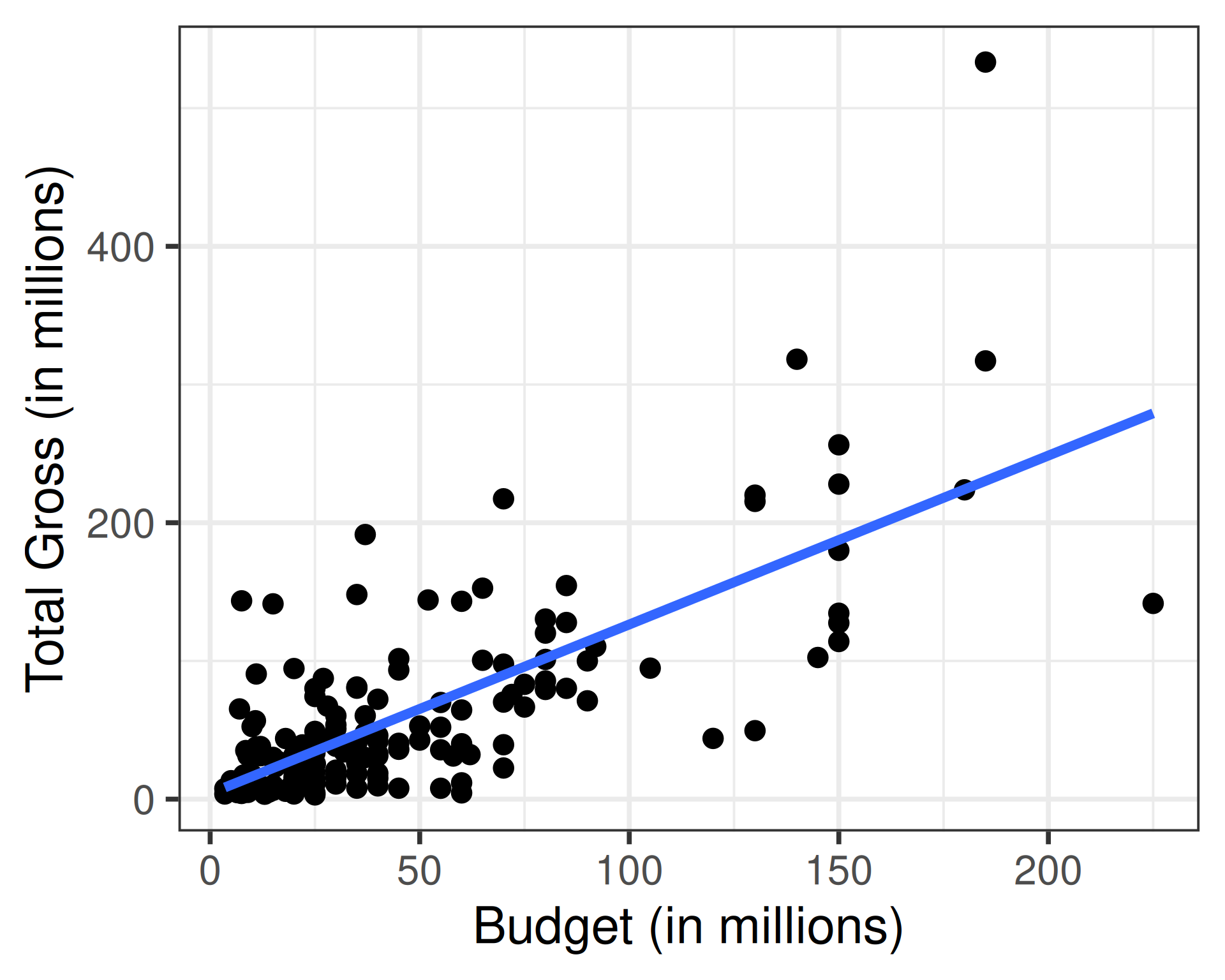
Given that Quantum of Solace cost $200,000,000 to produce, what do we predict its total box office gross to be?
Transformed model
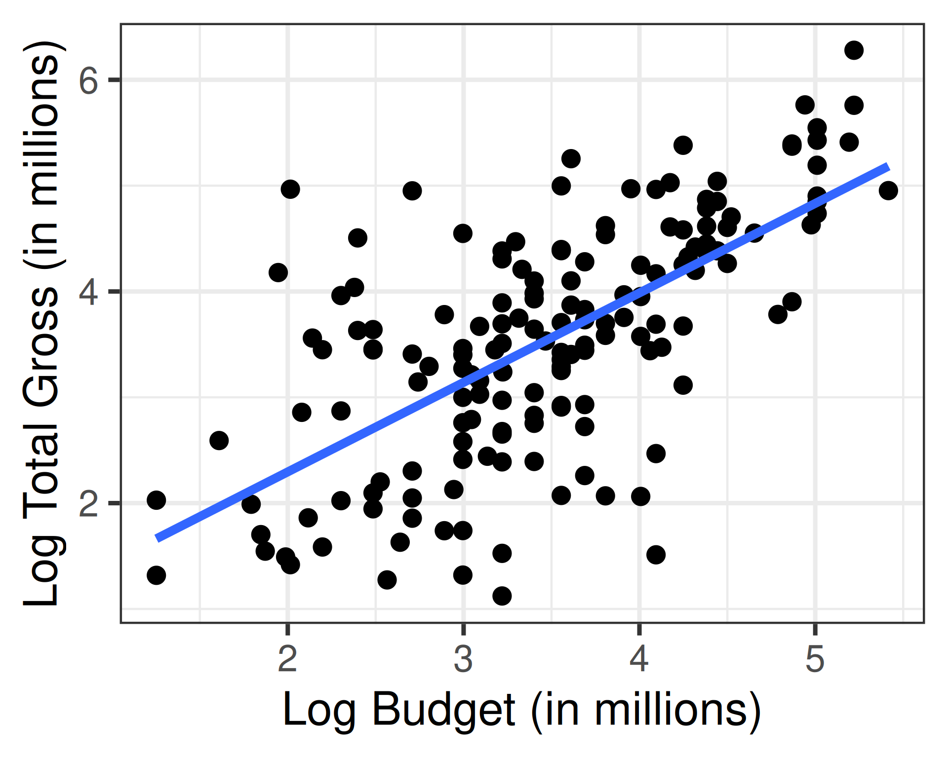
Let \(x_i\) be the budget and \(y_i\) the total box office gross of the \(i\)th movie, both in millions of dollars. Then:
\[\widehat{\log(y_i)} = 0.604 + 0.846\log(x_i)\]
Working with transformed models
\[ \log(Y_i) = \beta_0 + \beta_1\log(x_i) + \epsilon_i, \quad\text{where } \epsilon_i \overset{iid}{\sim} N(0, \sigma) \]
We still like to draw inferences about the broader population on the untransformed scales:
- Is there a relationship between \(x\) and \(Y\) in the broader population?
- How large is this relationship?
- What is the average value of \(Y\) in the subpopulation with \(x = x^*\)?
- What is the predicted value of \(Y\) for an individual with \(x = x^*\)?
Hypothesis Testing
Transformations/re-expressions won’t create new relationships where there were none previously!
- \(\rightarrow\) If \(f(Y)\) is not associated with \(g(x)\), then \(Y\) is not associated with \(x\)
- \(\therefore\) We can test \(H_0: \beta_1 = 0\) in our transformed model to learn whether a relationship exists between the untransformed variables!
Prediction of a Future Response
Regardless of what transformation of the response variable we used to make our prediction, we will want to re-express the prediction back on the original data scale (by applying the inverse transformation)
# A tibble: 1 × 4
  Budget_M .fitted .lower .upper
     <dbl>   <dbl>  <dbl>  <dbl>
1      200    5.08   3.36   6.81
Prediction of a Future Response
# A tibble: 1 × 3
  .fitted .lower .upper
    <dbl>  <dbl>  <dbl>
1    162.   28.9   903.
Working with transformed models
Inferences 2 and 3 require more careful consideration, since they aim to make statements about the population model for the mean: \[\begin{alignat*}{2} &\text{General:} &&E[f(Y) | g(x)] = \beta_0 + \beta_1 g(x)\\[0.75em] &\text{Movies in 2008:} \quad &&E[\log(Y) | \log(x)] = \beta_0 + \beta_1\log(x) \end{alignat*}\]
Interpretations for transformed variables can be clunky:
- E.g., \(g(x) = \sqrt{x}\): What does a one unit increase in the square root of a movie budget mean in practice?
- E.g., \(f(Y) = Y^{-1}\): How meaningful is a change in the average reciprocal of movie gross (measured in dollars\(^{-1}\))?
Interpreting log-transformed models
Note
\(\log\) transformations have the benefit of offering us convenient, sensical interpretations in terms of the original, untransformed variables!
The exact interpretation depends on which variable(s) was (were) transformed:
- The explanatory variable alone
- The response variable alone
- Both the explanatory and response variables
Aside: types of changes
The slope of a regression line tell us how a change in \(x\) relates to a constant change in (the mean of) \(y\)
- These changes can happen on additive or multiplicative scales
- Additive change: we always add the same constant \(c\)
- Multiplicative change: we always multiply by the same constant \(c\)
- The type of change in \(x\) that produces a constant type of change in \(y\) is a built in feature/assumption of the model
If only \(x\) is log-transformed
Because logarithms turn multiplication into addition, our interpretation of the slope will be in terms of multiplicative changes in \(x\):
- Model for the Mean: \(\mathbb{E}[Y | log(x)] = \beta_0 + \beta_1\log(x)\)
- Interpretation:
A \(c\)-fold multiplicative change in the explanatory variable is associated with a \(\beta_1\log(c)\) unit [increase/decrease] in the average value of the response variable.
Tip
The choice of \(c\) should depends on what scale of change makes sense for the data! A doubling? Then set \(c = 2\). A 10-fold change? Set \(c = 10\). A 10% reduction? Set \(c = 0.9\).
Example: if only \(x\) is log-transformed
The Happy Planet Index measures human well-being and environmental impact. Their data on a country’s GDP per capita (\(x\)) and life expectancy (\(y\)) is best summarized by the fitted linear model \[\widehat{y}_i = 20.12 + 5.62\log(x_i)\]
                     Estimate Std. Error   t value     Pr(>|t|)
(Intercept)         20.120197  2.4865124  8.091734 2.093958e-13
log(GDP_per_capita) 5.619668 0.2617096 21.472914 4.992533e-47Interpretation
A three-fold increase in GDP per capita is associated with an estimated 6.17 year increase in average life expectancy.
If only \(Y\) is log-transformed
Part of our goal when we transformed \(Y\) was to ensure that the resulting \(\log(Y)\) was symmetrically distributed about the regression line. This means the mean and the median of \(\log(Y)\) are the same! So our interpretation focuses on multiplicative changes in the median of \(Y\):
- Model for the Mean: \(\mathbb{E}[\log(Y) | x] = \beta_0 + \beta_1x\) \(\iff Median\{\log(Y)|x\} = \beta_0 + \beta_1x\) \(\iff \log(Median\{Y|x\}) = \beta_0 + \beta_1x\) \(\iff Median\{Y | x\} = e^{\beta_0 + \beta_1x}\)
Interpretation
A one unit increase in the explanatory variable is associated with a multiplicative change of \(e^{\beta_1}\) in the median value of the response variable.
Example: if only \(Y\) is log-transformed
Using data collected by The World Bank in 2020, we find that the relationship between a country’s GDP per capita (\(y\)) and the percent of its population that lives in urban areas (\(x\)) is given by \[\widehat{\log(y_i)} = 6.37 + 0.04x_i \iff \widehat{Median(y_i)} = e^{6.37 + 0.04 x_i}\]
A one percentage point increase in the percent of the population living in urban areas is associated with an estimated multiplicative change of 1.04 in the median GDP per capita.
If both \(x\) and \(Y\) are log-transformed
When both \(x\) and \(Y\) are log-transformed, we combine the previous two approaches! We consider how multiplicative changes in \(x\) associate with multiplicative changes in the median of \(Y\):
- Model for the Mean: \(\mathbb{E}[\log(Y) | \log(x)] = \beta_0 + \beta_1\log(x)\) \(\iff Median\{\log(Y)|\log(x)\} = \beta_0 + \beta_1\log(x)\) \(\iff Median\{Y | \log(x)\} = e^{\beta_0 + \beta_1\log(x)}\) \(\iff Median\{Y | \log(x)\} = e^{\beta_0}x^{\beta_1}\)
Interpretation
A \(c\)-fold multiplicative change in the explanatory variable is associated with a multiplicative change of \(c^{\beta_1}\) in the median value of the response variable.

SDS 291