10-Model Explanatory Power

SDS 291

Prof. Baumer

October 8, 2025

Recap: interpreting log-transformed models

Summary

Model Change in \(x\) Change in \(Y\) Captured by
\((x, Y)\) Additive (\(+1\)) Additive (in the mean) \(\beta_1\)
\((\log x, Y)\) Multiplicative (\(\times c\)) Additive (in the mean) \(\beta_1\log(c)\)
\((x, \log Y)\) Additive (\(+1\)) Multiplicative (in the median) \(e^{\beta_1}\)
\((\log x, \log Y)\) Multiplicative (\(\times c\)) Multiplicative (in the median) \(c^{\beta_1}\)

Model explanatory power

Decomposing variability: ANOVA

  • Total variability (SST):
    • variability explained by the model (SSM)
    • unexplained variability in the residuals (SSE)

\[ SST = SSM + SSE \]
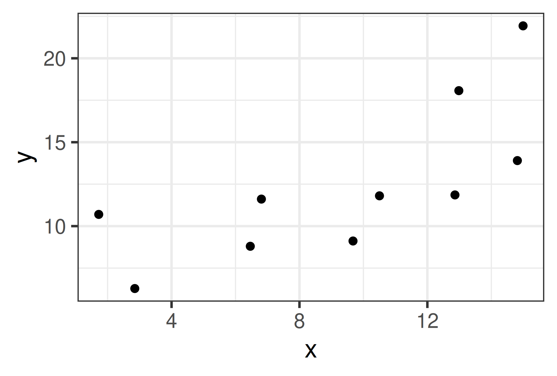
Decomposing variability: ANOVA

Total Sum of Squares
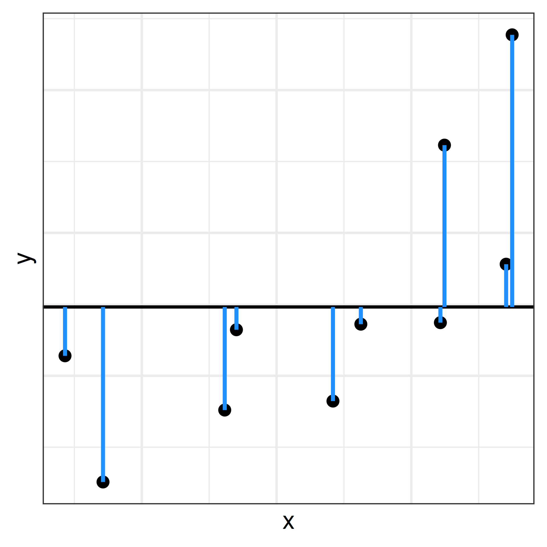
\[\begin{align*} SST &= \sum_{i=1}^{n}(y_i - \bar{y})^2\\[0.25em] df &= n - 1 \end{align*}\]

Model Sum of Squares
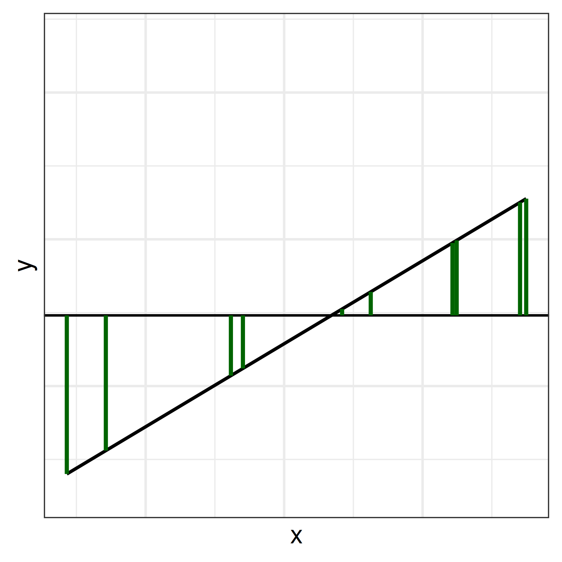
\[\begin{align*} SSM &= \sum_{i=1}^{n}(\widehat{y}_i - \bar{y})^2\\[0.25em] df &= 1 \end{align*}\]

Error Sum of Squares
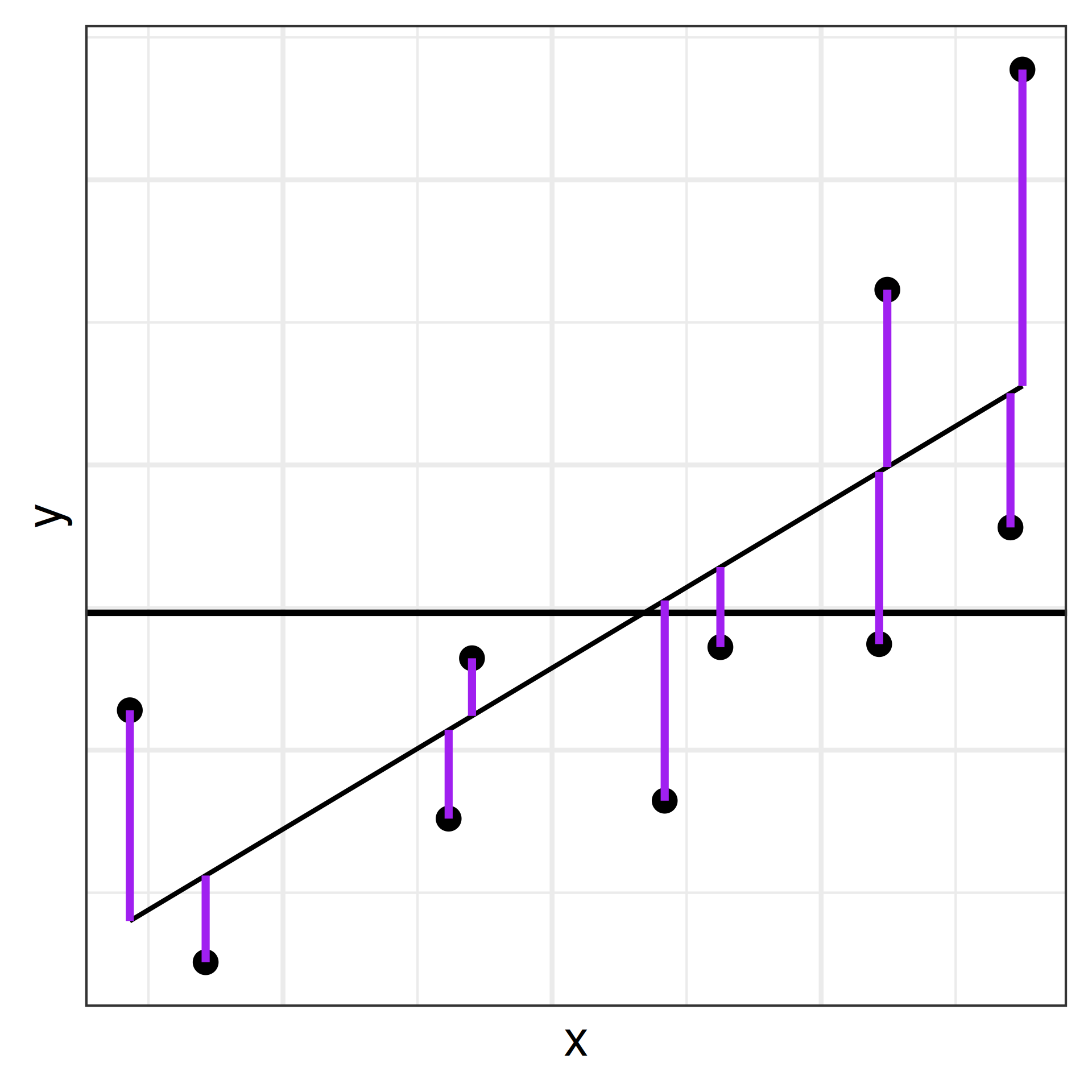
\[\begin{align*} SSE &= \sum_{i=1}^{n}(y_i - \widehat{y}_i)^2\\[0.25em] df &= n - 2 \end{align*}\]

Uses of ANOVA: \(F\)-tests

We use ANOVA to assess the explanatory/predictive power of our model in three ways:

  1. (In a few weeks) To conduct hypothesis tests comparing two possible models for the data

Uses of ANOVA: mean squared error

  1. Mean Squared Error (\(MSE\)):
    • Average distance between the model’s prediction (\(\widehat{y}_i\)) and the truth (\(y_i\))
    • Equal to the sample variance of the residuals, \(e_i\),…
    • …estimates the variance of the population error terms, \(\epsilon_i\): \[MSE = \frac{\sum_{i=1}^{n}(y_i - \widehat{y}_i)^2}{n-2} = \frac{SSE}{n-2} = \widehat{\sigma_{\epsilon}}^2\]
    • Root mean square error (RMSE, a.k.a. residual standard deviation): \[\widehat{\sigma_{\epsilon}} = \sqrt{MSE}\]

Using ANOVA: \(R^2\)

  1. coefficient of determination (\(R^2\)):
    • Answers the question “what proportion of the variability that we observe in \(Y\) can be explained by the linear regression of \(Y\) on \(x\)?” \[R^2 = \frac{SSM}{SST} = \frac{SST - SSE}{SST} = 1 - \frac{SSE}{SST}\]

Making Connections

The \(R^2\) gets its name from the fact that—for a simple linear regression model—it is exactly equal to the square of the Pearson correlation coefficient, \(r\), between \(x\) and \(y\)!

RMSE and \(R^2\) in R

The glance() function in the broom package:

  • r.squared: the coefficient of determination, \(R^2\)
  • sigma: the RMSE, \(\widehat{\sigma_{\epsilon}}\)
  • df: the model degrees of freedom
  • df.residual: the residual degrees of freedom, \(n - 2\)
library(broom)
ll_movies_lm |>
  glance() |>
  select(c("r.squared", "sigma", "df", "df.residual"))
# A tibble: 1 × 4
  r.squared sigma    df df.residual
      <dbl> <dbl> <dbl>       <int>
1     0.435 0.858     1         158

Note

How would we interpret this \(R^2\) value in context?

Root MSE and \(R^2\) in R

summary(ll_movies_lm)

Call:
lm(formula = log(Total_Gross/1e+06) ~ log(Budget_2008/1e+06), 
    data = movies_08)

Residuals:
     Min       1Q   Median       3Q      Max 
-2.55463 -0.56476  0.04446  0.55762  2.65824 

Coefficients:
                       Estimate Std. Error t value Pr(>|t|)    
(Intercept)             0.60419    0.27506   2.197   0.0295 *  
log(Budget_2008/1e+06)  0.84563    0.07669  11.027   <2e-16 ***
---
Signif. codes:  0 '***' 0.001 '**' 0.01 '*' 0.05 '.' 0.1 ' ' 1

Residual standard error: 0.8577 on 158 degrees of freedom
  (46 observations deleted due to missingness)
Multiple R-squared:  0.4349,    Adjusted R-squared:  0.4313 
F-statistic: 121.6 on 1 and 158 DF,  p-value: < 2.2e-16