11-Multiple Linear Regression

SDS 291

Prof. Baumer

October 8, 2025

The multiple linear regression model

What has changed?

Multiple Linear Regression

\[ Y_i = \beta_0 + \beta_1 x_{i1} + \beta_2 x_{i2} + \cdots + \beta_k x_{ik} + \epsilon, \quad\text{where } \epsilon_i \overset{iid}{\sim} N(0, \sigma) \]

  1. We have more terms!
  2. Interpretation of model parameters has to be adjusted
    • Now in relation to (i.e., conditional on) the other variables
  3. We estimate more parameters: \(k\) slopes and one intercept
    • Model degrees of freedom: \(k\)
    • Residual degrees of freedom: \(n - (k + 1) = n - k - 1\)
    • Mean squared error: \(\widehat{\sigma_\epsilon}^2 = SSE/(n - k - 1)\)
    • \(p\)-values, CIs, PIs calculated using a \(t_{n-k-1}\) distribution

What has stayed the same?

Pretty much everything else!

  1. Fit the model by minimizing sum of squared residual error
  2. Require same conditions on \(\epsilon_i\) for \(t\)-based inference
  3. Approach to hypothesis tests, CIs, PIs remains the same
    • just with a different \(t\)-distribution
  4. \(R^2\) still captures the proportion of variability model explains

What do we mean by “linear”?

Note

Which of the following mathematical models for the mean are examples of multiple linear regression models?

  1. \(\mathbb{E}[Y | x_1, x_2] = \beta_0 + \beta_1 \log(x_1) + \beta_2 \log(x_2)\)
  2. \(\mathbb{E}[Y | x_1, x_2] = e^{\beta_0 + \beta_1 x_1 + \beta_2 x_2}\)
  3. \(\mathbb{E}[Y | x_1] = \beta_0 + \beta_1 x_1 + \beta_2 x_1^2\)
  4. \(\mathbb{E}[Y | x_1, x_2] = \beta_0 + \beta_1 x_1 + \beta_2 x_2 + \beta_3x_1x_2\)

Tip

  • “linear” means linear in the parameters (i.e., the regression coefficients)!
  • The resulting regression surface may look highly non-linear in terms of the original explanatory variables!

Example: Palmer penguins

Scientists collected body measurements (including flipper length, body mass, and bill dimensions) for 344 adult foraging penguins sampled from the Palmer Archipelago in Antarctica

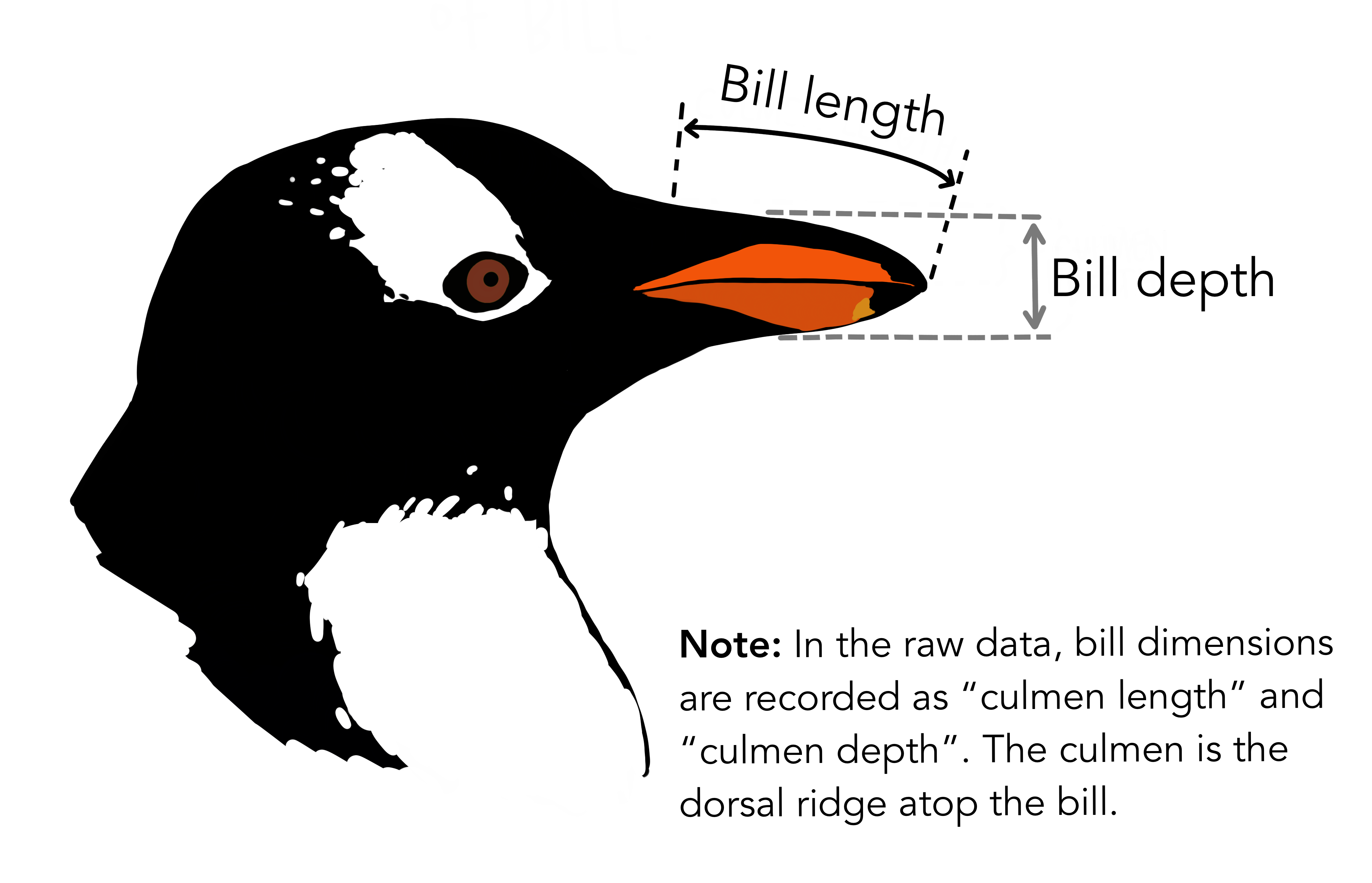
Example: Palmer penguins
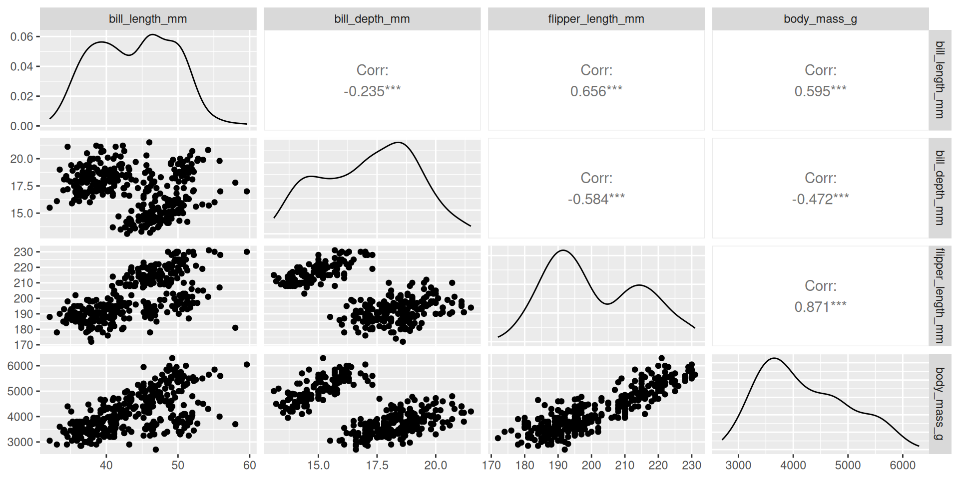
library(palmerpenguins)
penguins |>
  select(contains("_mm"), contains("_g")) |>
  GGally::ggpairs()

The march of the penguins

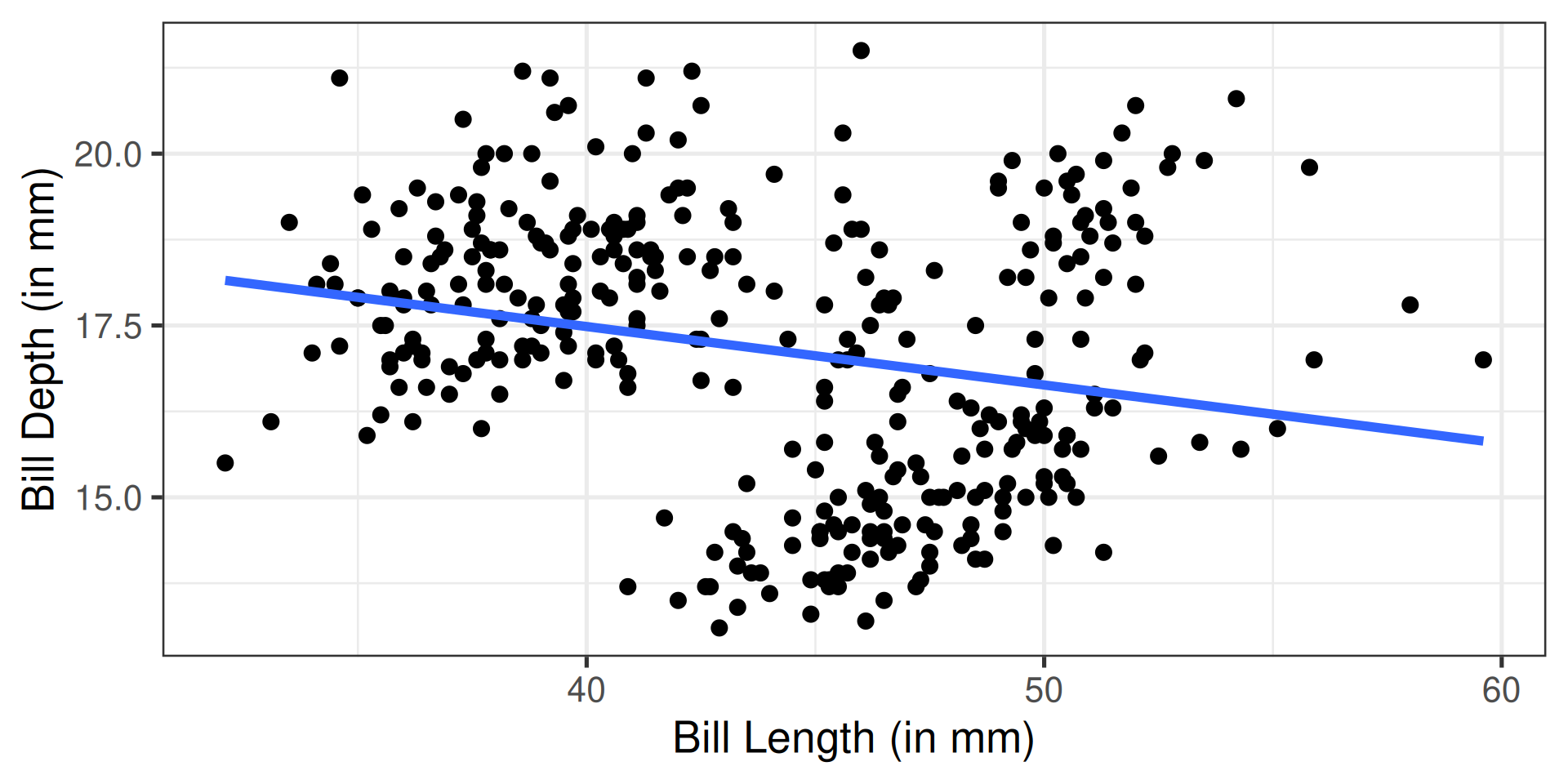
How does a penguin’s expected bill depth (in mm) change as a function of its bill length (in mm)?

\[ \widehat{depth} = 20.89 - 0.09 \cdot \left( bill \right) \]
The emperor (penguin) strikes back

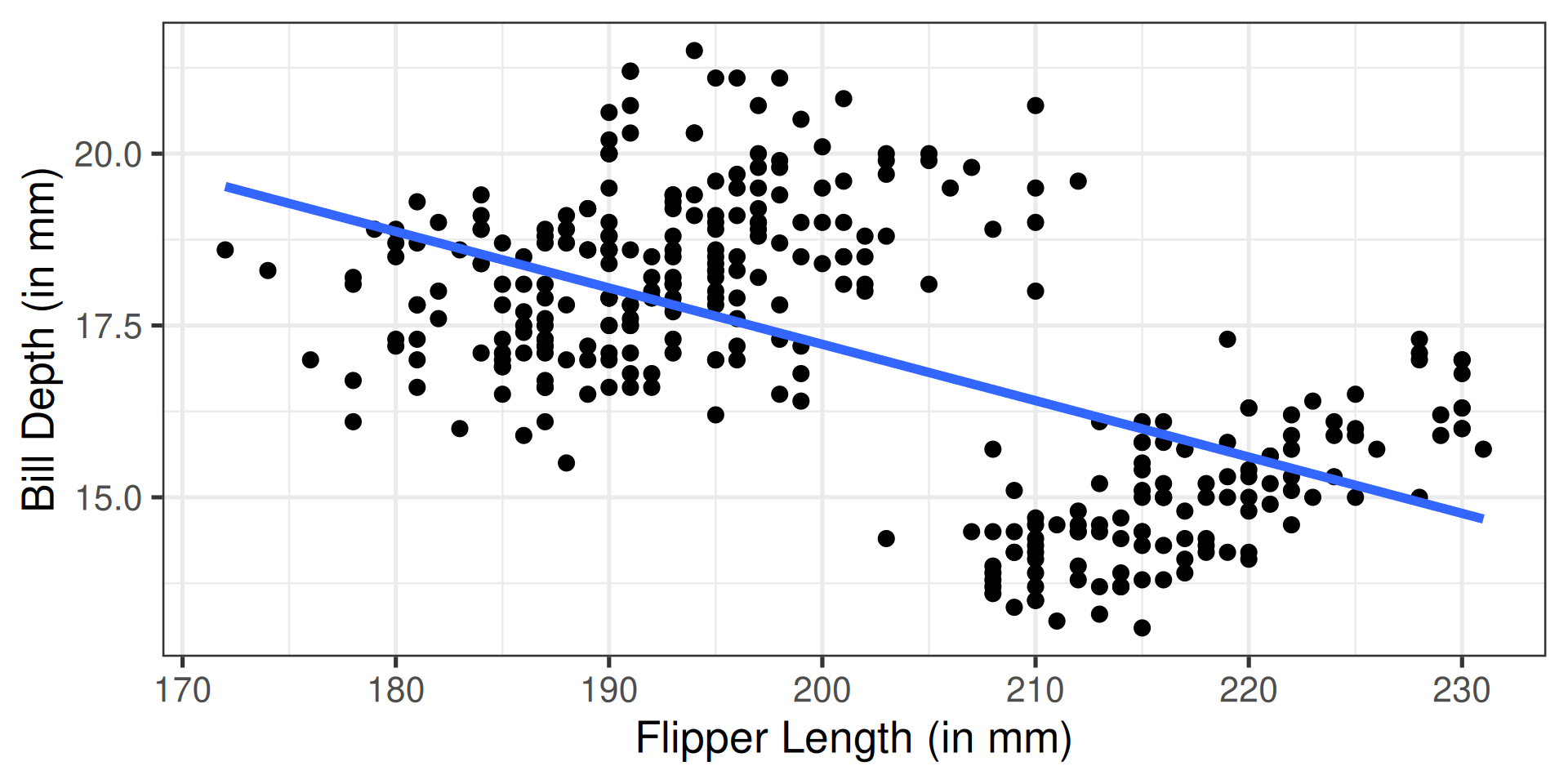
How does a penguin’s expected bill depth (in mm) change as a function of its flipper length (in mm)?

\[ \widehat{depth} = 33.63 - 0.08 \cdot \left( flipper \right) \]
A colony of penguin variables

How does a penguin’s expected bill depth (in mm) change as a function of both its bill length (in mm) and its flipper length (in mm)?

\[ \widehat{depth} = 34.31 + 0.09\cdot \left( bill \right) - 0.11 \cdot \left( flipper \right) \]

Visualizing the model

Fitting MLR in R

mod_mlr <- lm(bill_depth_mm ~ bill_length_mm + flipper_length_mm, data = penguins)
summary(mod_mlr)

Call:
lm(formula = bill_depth_mm ~ bill_length_mm + flipper_length_mm, 
    data = penguins)

Residuals:
    Min      1Q  Median      3Q     Max 
-3.0875 -1.1351 -0.0724  1.0879  4.5167 

Coefficients:
                   Estimate Std. Error t value Pr(>|t|)    
(Intercept)       34.308407   1.219366  28.136  < 2e-16 ***
bill_length_mm     0.094050   0.020510   4.586 6.38e-06 ***
flipper_length_mm -0.105956   0.007963 -13.306  < 2e-16 ***
---
Signif. codes:  0 '***' 0.001 '**' 0.01 '*' 0.05 '.' 0.1 ' ' 1

Residual standard error: 1.56 on 339 degrees of freedom
  (2 observations deleted due to missingness)
Multiple R-squared:  0.3794,    Adjusted R-squared:  0.3757 
F-statistic: 103.6 on 2 and 339 DF,  p-value: < 2.2e-16

Why multiple regression?

  1. Summarize a pattern observed in the data
    • Less relevant for multiple linear regression models
    • Visualizing models with multiple explanatory variables is awkward and often unfeasible
  2. Classify or predict values of an outcome of interest
    • Incorporating additional relevant explanatory variables will hopefully improve our prediction!
  3. Quantify and evaluate the strength of relationships between variables
    • Relationships now adjusted for other variables (e.g., known confounders)!
    • We can also capture more complex and more flexible relationships between the variables
  4. Address violations of the linearity condition

Example: SLR for prediction

Research Question

What is the predicted bill length for an individual penguin on the Palmer archipelago with a bill length of 50 mm and flipper length of 195 mm?
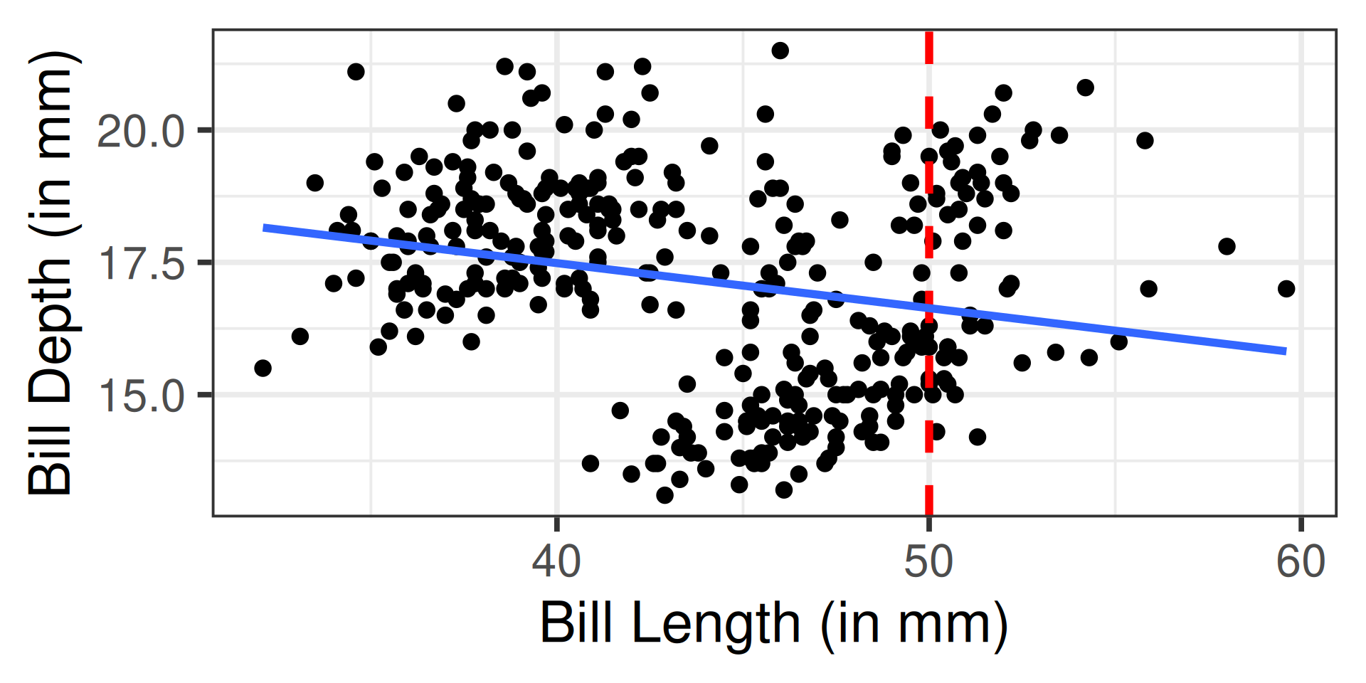
new_bird <- data.frame(flipper_length_mm = 195, bill_length_mm = 50)

PI from SLR model

mod_slr <- lm(bill_depth_mm ~ bill_length_mm,
  data = penguins
)

mod_slr |>
  broom::augment(
    newdata = new_bird,
    interval = "prediction",
    conf.level = 0.95
  ) |>
  select(c(".fitted", ".lower", ".upper"))
# A tibble: 1 × 3
  .fitted .lower .upper
    <dbl>  <dbl>  <dbl>
1    16.6   12.8   20.4
  • Prediction interval has a width of \(20.4 - 12.8 = 7.6\)mm

Example: MLR for prediction

PI from MLR model

mod_mlr |>
  broom::augment(
    newdata = new_bird,
    interval = "prediction",
    conf.level = 0.95
  ) |>
  select(c(".fitted", ".lower", ".upper"))
# A tibble: 1 × 3
  .fitted .lower .upper
    <dbl>  <dbl>  <dbl>
1    18.3   15.3   21.4
  • The prediction has changed!
  • This prediction interval has a width of \(21.4 - 15.3 = 6.1\)mm!