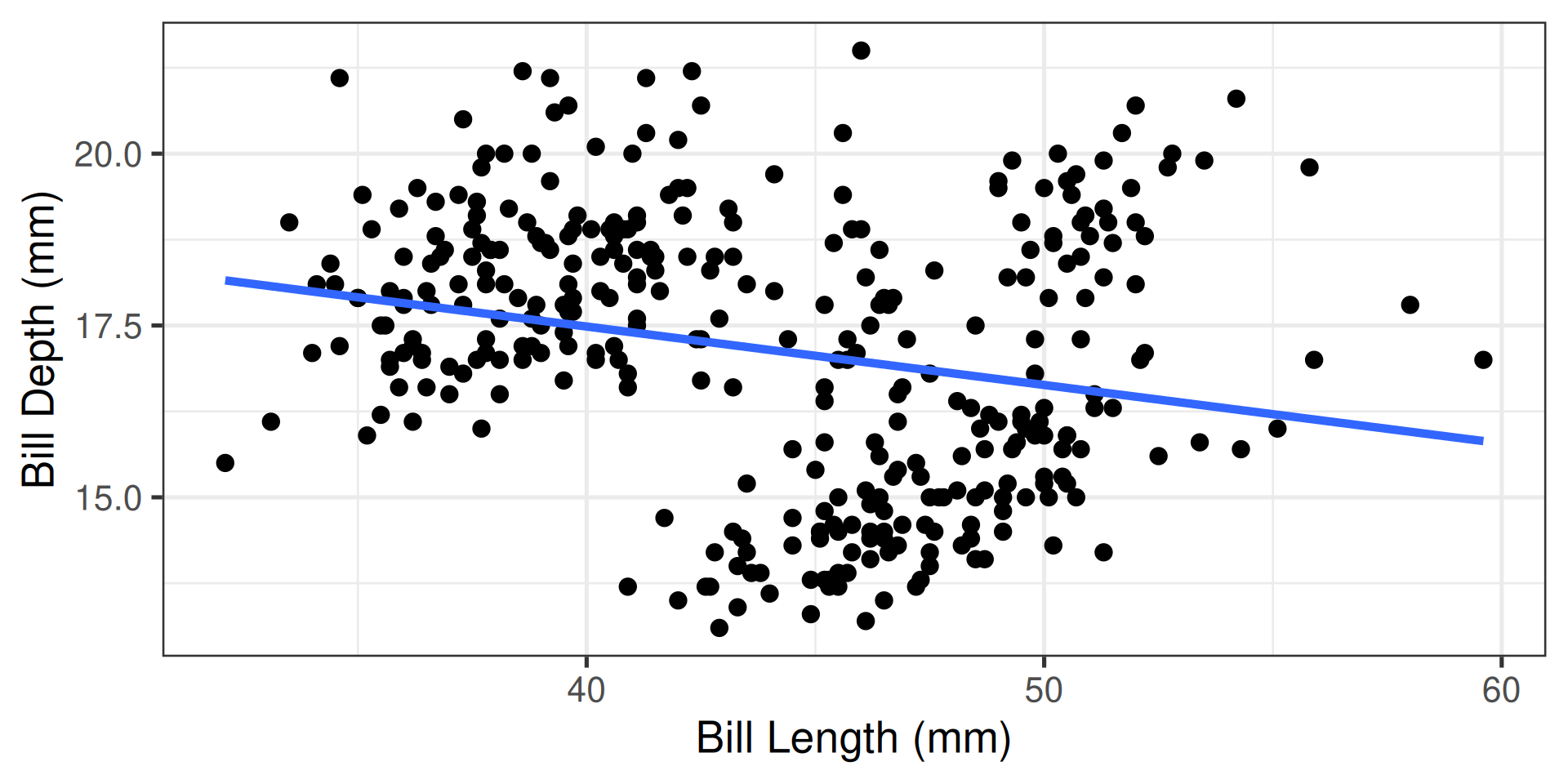
                  Estimate Std. Error   t value     Pr(>|t|)
(Intercept)    20.88546832 0.84388321 24.749240 4.715137e-78
bill_length_mm -0.08502128 0.01906694 -4.459093 1.119662e-0512-MLR with Categorical Variables
SDS 291
Prof. Baumer
October 15, 2025
Ex: MLR for estimating associations
Research Question
What is the association between the bill depth and bill length of Antarctic penguins?
Simple Linear Regression
Multiple Linear Regression
                     Estimate  Std. Error    t value     Pr(>|t|)
(Intercept)       34.30840672 1.219365662  28.136274 1.104331e-90
bill_length_mm     0.09405042 0.020509566   4.585686 6.375054e-06
flipper_length_mm -0.10595571 0.007963019 -13.305972 8.593353e-33
Confounders
- Variables that are associated with both the explanatory variable of interest, \(x\), and the response variable, \(Y\)
- If not accounted for, can result in seeing a spurious or distorted relationship between \(x\) and \(Y\)
- Not accounting for confounders means that our simple linear regression slope represents an “apples to oranges” comparison of penguin subpopulations, rather than an “apples to apples” comparison
Ice cream and crime
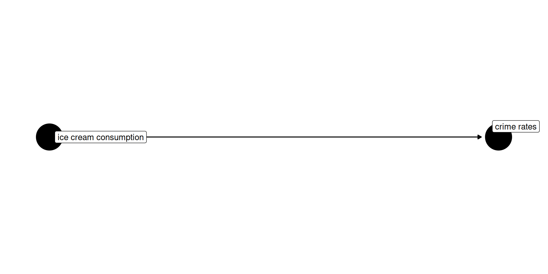
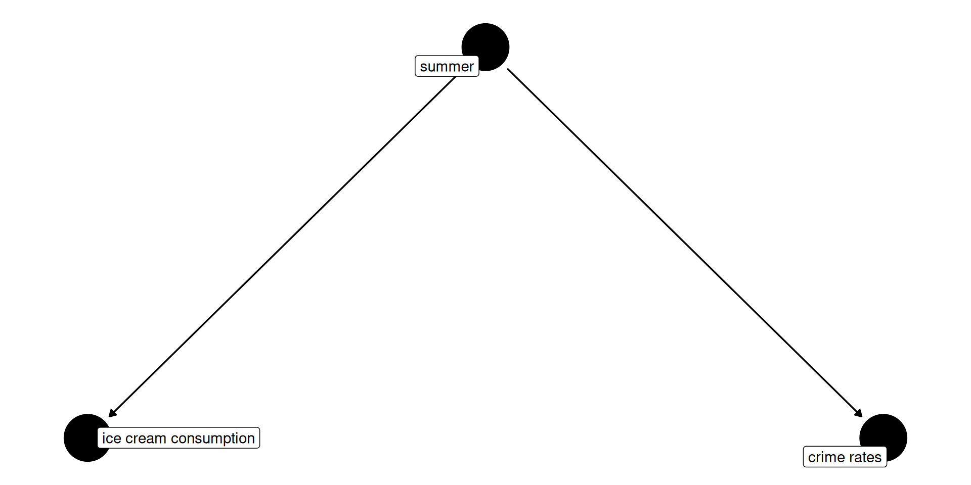
What’s going on behind the scenes?
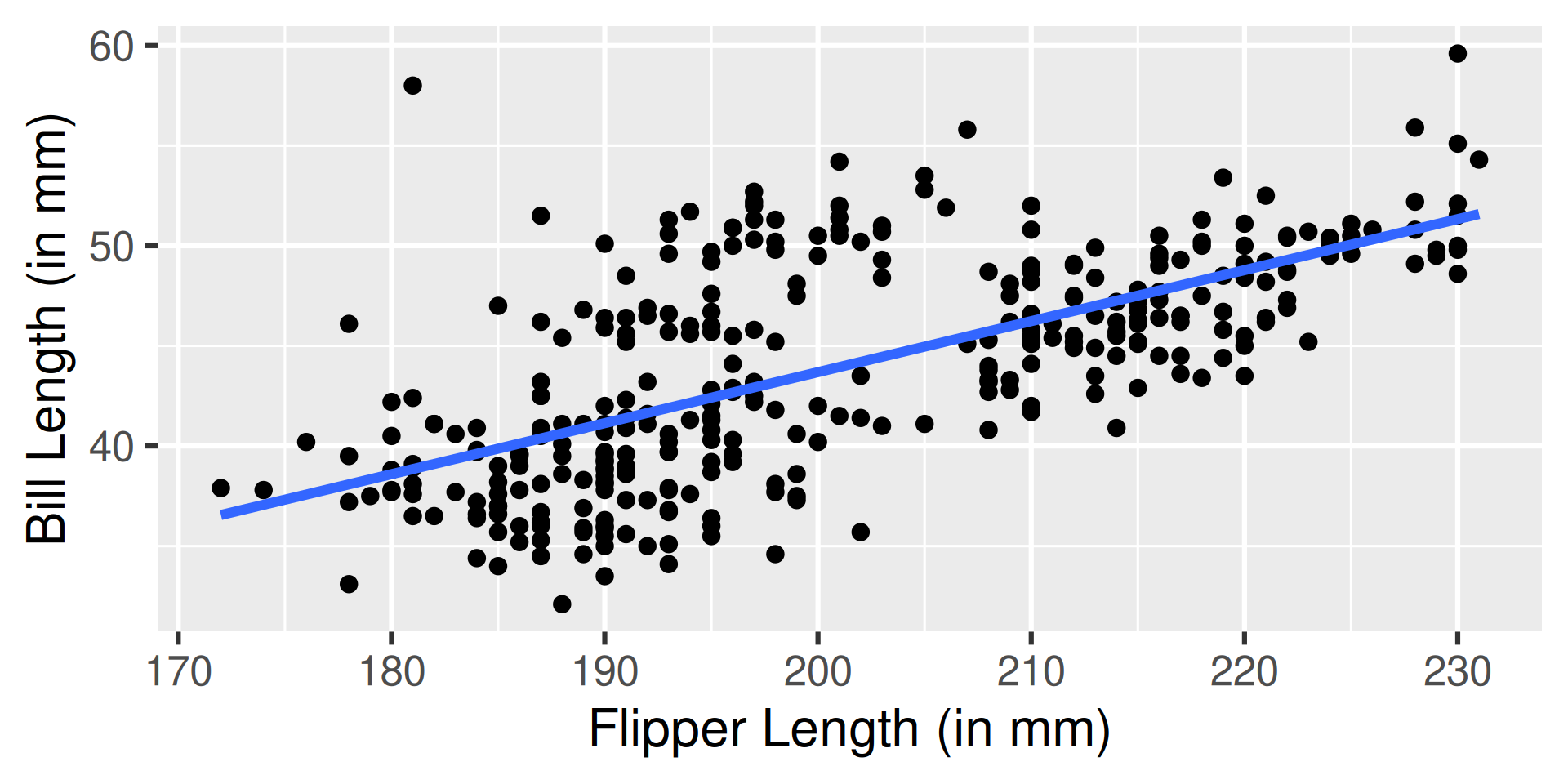
- Bill length and flipper length have their own relationship!
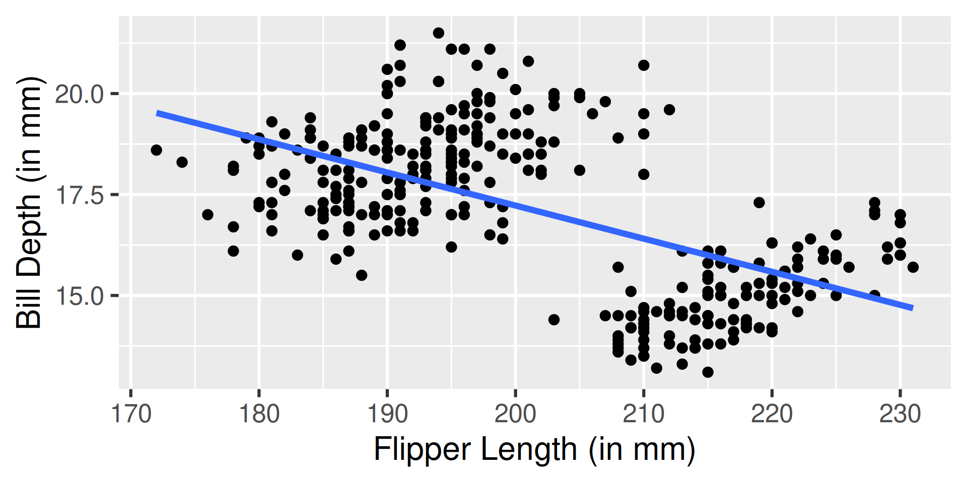
- …as do flipper length and bill depth
- Penguins with longer flippers tend to have longer bills…
- …and penguins with longer flippers also tend to have shallower bills!
MLR Interpretations
General Form of a Multiple Regression Model for the Mean
\[E[Y|x_1, x_2] = \beta_0 + \beta_1x_1 + \beta_2 x_2\]
- Intercept: the mean value of the response variable when both explanatory variables are set equal to zero
- \(E[Y|x_1 = 0, x_2 = 0] = \beta_0 + \beta_1(0) + \beta_2(0) = \beta_0\)
- Slope: the change in the mean value of the response variable associated with a one unit increase in the explanatory variable, holding all other explanatory variables in the model constant
- \(E[Y|x_1 = x_1^*, x_2 = x_2^*] = \beta_0 + \beta_1x_1^* + \beta_2x_2^*\)
- \(\begin{align*} E[Y|x_1 = x_1^* + 1, x_2 = x_2^*] &= \beta_0 + \beta_1(x_1^* + 1) + \beta_2x_2^* \\ &= \beta_0 + \beta_1x_1^* + \mathbf{\beta}_1 + \beta_2x_2^* \end{align*}\)
Ex: interpreting the penguin model
\[ \widehat{\texttt{depth}} = 34.31 + 0.09\left(\texttt{bill}\right) - 0.11\left(\texttt{flipper}\right) \]
- Intercept: The mean bill depth of penguins with a bill length of 0 mm and a flipper length of 0 mm is estimated to be 34.31 mm.
- Typically not meaningful to interpret!
- Slope for \(x_1\): After controlling for flipper length, a one mm increase in bill length is associated with an estimated 0.09 mm increase in the mean bill depth of Antarctic penguins.
- Slope for \(x_2\): A one mm increase in flipper length is associated with an estimated 0.11 mm decrease in the mean bill depth, holding penguin bill length constant.
Ex: inference with confounders
Research Question
What is the association between the bill depth and bill length of Antarctic penguins, holding penguin flipper length constant?
                        2.5 %      97.5 %
(Intercept)       31.90993097 36.70688247
bill_length_mm     0.05370838  0.13439246
flipper_length_mm -0.12161886 -0.09029256
Interpretation
We are 95% confident that a one mm increase in bill length is associated with between a 0.05 mm and 0.13 mm increase in mean bill depth among Antarctic penguins, holding penguin flipper length constant.
Ex: testing with confounders
Research Question
Is there a linear relationship between the bill depth and bill length of Antarctic penguins, after accounting for penguin flipper length?
- \(H_0\): \(\beta_1 = 0\), given the other variables in the model
- \(H_A\): \(\beta_1 \neq 0\), given the other variables in the model
                     Estimate  Std. Error    t value     Pr(>|t|)
(Intercept)       34.30840672 1.219365662  28.136274 1.104331e-90
bill_length_mm     0.09405042 0.020509566   4.585686 6.375054e-06
flipper_length_mm -0.10595571 0.007963019 -13.305972 8.593353e-33
Interpretation
After controlling for the effects of penguin flipper length, there is a statistically significant relationship between the bill depth and bill length of Antarctic penguins (\(p < 0.001\)).
Example: other confounders?
Note
What other factors might confound the relationship between bill depth and bill length?
Indicator variables
Indicators: use two values, usually 0 and 1, to indicate whether an observation does (1) or does not (0) belong to a particular category
- Categorical variable with \(k\) levels requires \(k-1\) indicator variables
- Omitted level is called the reference level
Binary indicator variable
Binary Categorical Variable (\(k = 2\))
Can represent a penguin’s sex using one indicator: \[ \texttt{Male}_i = \begin{cases} \ 1 & \text{if penguin }i\text{ is male}\\ \ 0 & \text{if penguin }i \text{ is not male} \end{cases} \]
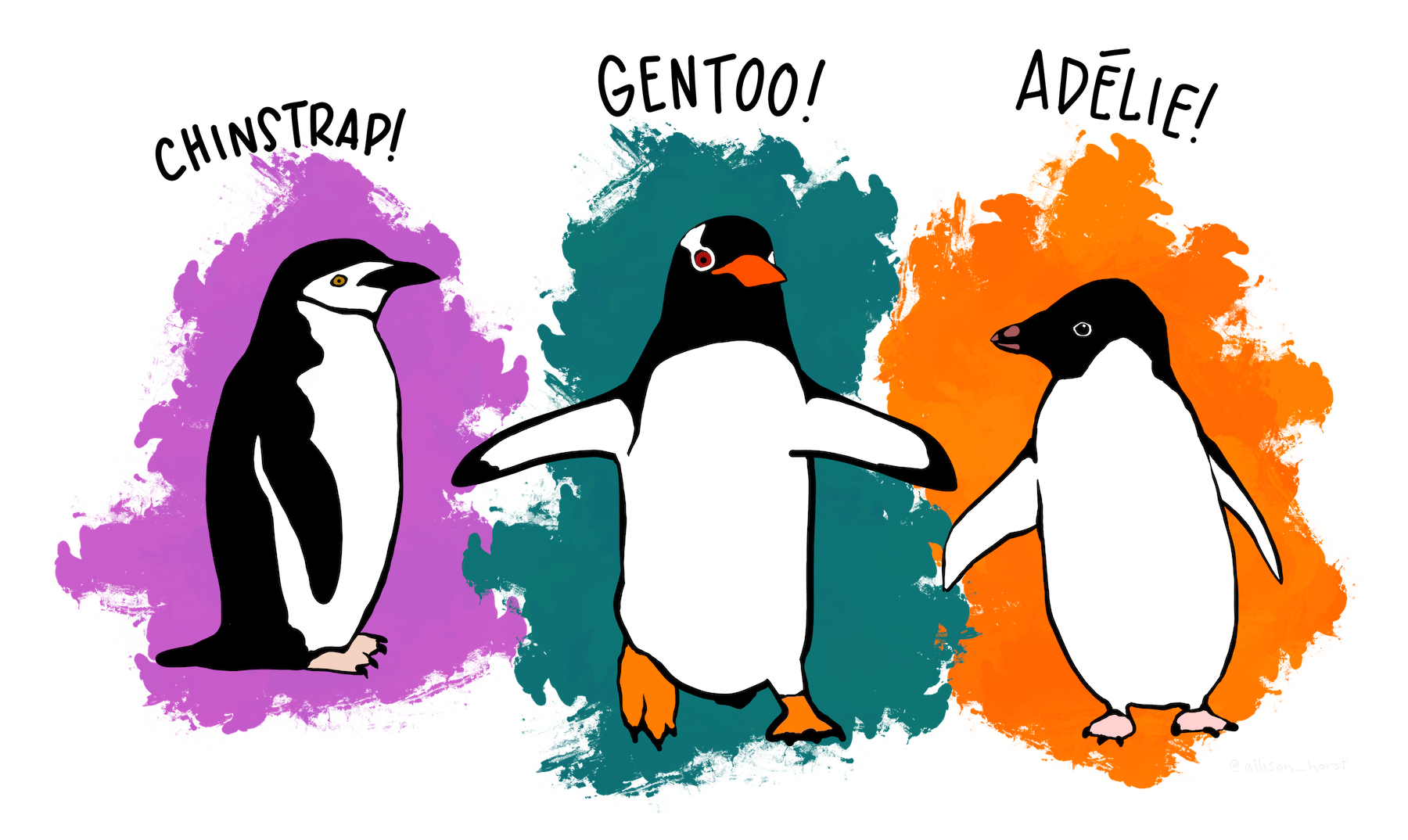
Three species
Categorical indicator variable
Categorical Variable (\(k > 2\))
Can represent the three penguin species found in the Palmer Archipelago (Adelie, Chinstrap, and Gentoo) using two indicators: \[\begin{align*} \texttt{Adelie}_i &= \begin{cases} \ 1 & \text{if penguin }i\text{ is a Adelie penguin}\\ \ 0 & \text{otherwise} \end{cases}\\ \texttt{Gentoo}_i &= \begin{cases} \ 1 & \text{if penguin }i\text{ is a Gentoo penguin}\\ \ 0 & \text{otherwise} \end{cases} \end{align*}\]
Categorical explanatory variables in R
Represented by factor variables:
- The levels (i.e., possible values/categories)
- The reference level
[1] "Adelie" "Chinstrap" "Gentoo" Fitting models with cat. variables in R
lm() automatically creates indicators for any factor
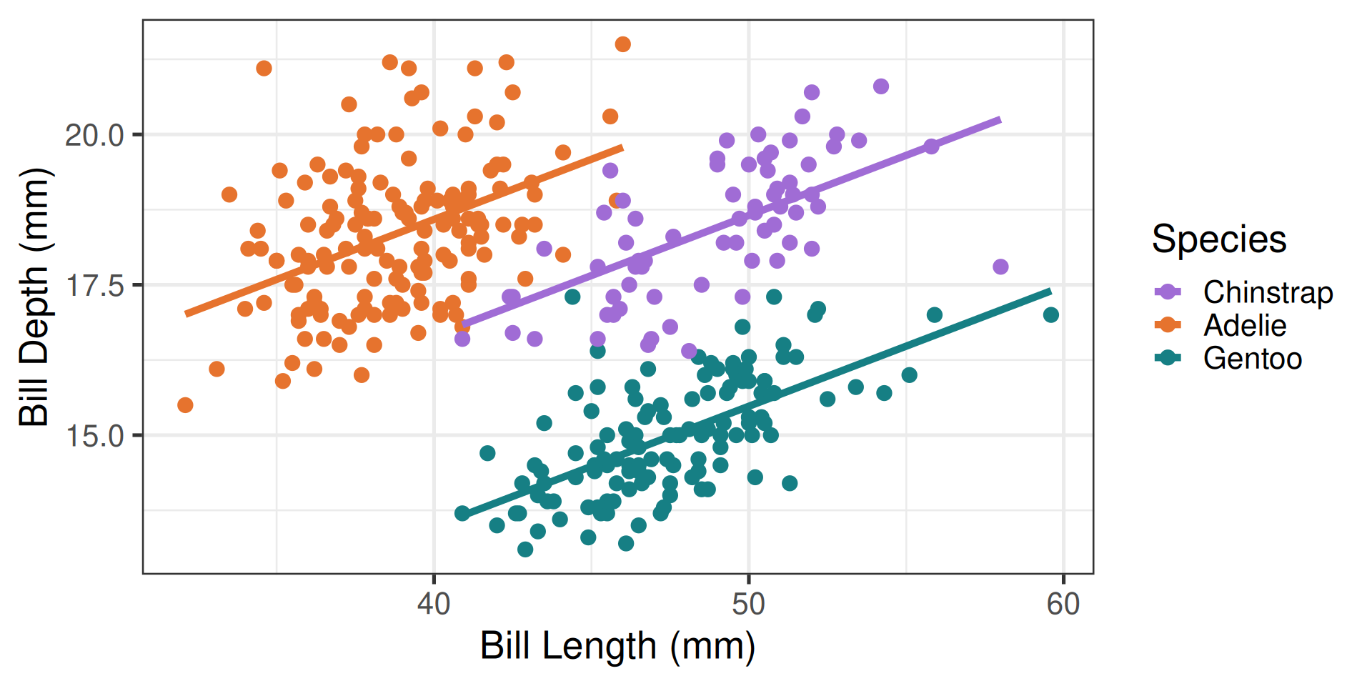
                 Estimate Std. Error   t value     Pr(>|t|)
(Intercept)     8.6589862 0.86206892  10.04442 6.039045e-21
bill_length_mm  0.1998943 0.01749365  11.42668 8.661124e-26
speciesAdelie   1.9331943 0.22416005   8.62417 2.545386e-16
speciesGentoo  -3.1728258 0.14592926 -21.74222 3.473444e-66
Fitted Model
\[\widehat{y} = 8.66 + 0.20x_1 + 1.93x_2 - 3.17 x_3\]
Visualizing the model

SDS 291