14-MLR with Polynomials

SDS 291

Prof. Baumer

October 22, 2025

Interaction models

Ex: Penguin size

Suppose we wanted to understand the relationship between penguin bill length (in mm), flipper length (in mm), and body mass (in g):

Population Model for the Mean: \[ \mathbb{E}[\texttt{mass}_i | \texttt{bill}_i, \texttt{flipper}_i] = \beta_0 + \beta_1\left(\texttt{bill}_i\right) + \beta_2\left(\texttt{flipper}_i\right) \]

Fitted Regression Model:

mod_mass <- lm(body_mass_g ~ bill_length_mm + flipper_length_mm, data = penguins)
broom::tidy(mod_mass)

# A tibble: 3 × 5
  term              estimate std.error statistic  p.value
  <chr>                <dbl>     <dbl>     <dbl>    <dbl>
1 (Intercept)       -5737.      308.      -18.6  7.80e-54
2 bill_length_mm        6.05      5.18      1.17 2.44e- 1
3 flipper_length_mm    48.1       2.01     23.9  7.56e-75

Example: Palmer penguins

Visualization of model

Interactions btw 2 numeric variables

If we allow for a possible interaction between bill length and flipper length, then the population model becomes \[\begin{align*} \mathbb{E}[\texttt{mass}_i | \texttt{bill}_i, \texttt{flipper}_i] &= \beta_0 + \beta_1\left(\texttt{bill}_i\right) + \beta_2\left(\texttt{flipper}_i\right) \\ &+ \beta_3\left(\texttt{bill}_i\right)\left(\texttt{flipper}_i\right) \end{align*}\]

Once again, relationships are no longer captured by a single parameter:

Overall slope \(\iff\) relationship between bill length and body mass \[\left( \beta_1 + \beta_3 \left( \texttt{flipper}_i\right) \right) \left( \texttt{bill}_i \right)\]
Overall slope \(\iff\) relationship between flipper length and body mass \[\left( \beta_2 + \beta_3 \left( \texttt{bill}_i \right) \right) \left( \texttt{flipper}_i \right)\]

Fitting an interaction model

mod_mass_int <- lm(body_mass_g ~ bill_length_mm * flipper_length_mm, data = penguins)
summary(mod_mass_int)


Call:
lm(formula = body_mass_g ~ bill_length_mm * flipper_length_mm, 
    data = penguins)

Residuals:
     Min       1Q   Median       3Q      Max 
-1040.18  -283.07   -23.94   241.93  1241.40 

Coefficients:
                                  Estimate Std. Error t value Pr(>|t|)    
(Intercept)                      5090.5088  2925.3007   1.740 0.082740 .  
bill_length_mm                   -229.2424    63.4334  -3.614 0.000347 ***
flipper_length_mm                  -7.3085    15.0321  -0.486 0.627145    
bill_length_mm:flipper_length_mm    1.1998     0.3224   3.721 0.000232 ***
---
Signif. codes:  0 '***' 0.001 '**' 0.01 '*' 0.05 '.' 0.1 ' ' 1

Residual standard error: 386.8 on 338 degrees of freedom
  (2 observations deleted due to missingness)
Multiple R-squared:  0.7694,    Adjusted R-squared:  0.7674 
F-statistic: 375.9 on 3 and 338 DF,  p-value: < 2.2e-16

Interactions result in a warped plane!

Interpreting the coefficients

\[\begin{align*} \widehat{\texttt{mass}}_i &= {\color{ProcessBlue}5090.51} -229.24\left(\texttt{bill}_i\right) -7.31\left(\texttt{flipper}_i\right) \\ &{\color{white}=} + 1.20\left(\texttt{bill}_i\right)\left(\texttt{flipper}_i\right) \end{align*}\]

intercept (\(\widehat{\beta}_0\)) represents the \(z\)-axis intercept of the warped plane:
- In context: the average body mass of a penguin with a bill length of 0 mm and a flipper length of 0 mm is 5,090.51 grams

Interpretting the main effect terms

coefficient for the main effect of bill length (\(\widehat{\beta}_1\)) represents the association between bill length and body mass when flipper length is 0 mm:
- In context: for each additional mm in bill length, the mean body mass of a penguin with a flipper length of 0 mm decreases by 229.24 grams
coefficient for the main effect of flipper length (\(\widehat{\beta}_2\)) represents the association between flipper length and body mass when bill length is 0 mm:
- In context: for each additional mm in flipper length, the mean body mass of a penguin with a bill length of 0 mm decreases by 7.31 grams

Interpretting the interaction terms

interaction term (\(\widehat{\beta}_3\)) once again captures the change in the slope:
- represents the change in the slope for bill length, for each additional one mm of flipper length
- represents the change in the slope for flipper length, for each additional one mm of bill length

Interpretation in practice

The “raw” coefficients of the numeric interaction model suffer the same fate as the intercept in other linear regression models:

Correspond to the (change in the) mean value of the response variable (e.g., penguin mass) for a subpopulation in which the other explanatory variables in the interaction are set equal to 0
Not very interpretable!

Instead

Typically calculate and interpret the change in the mean response for other, more meaningful values!

penguins |>
  summarize(
    mean_flipper_length = mean(flipper_length_mm, na.rm = TRUE),
    mean_bill_length = mean(bill_length_mm, na.rm = TRUE)
  )

# A tibble: 1 × 2
  mean_flipper_length mean_bill_length
                <dbl>            <dbl>
1                201.             43.9

Interpretion in practice

\[\begin{align*} \widehat{\texttt{mass}}_i &= 5090.51 -229.24 \left( \texttt{bill}_i \right) - 7.31 \left( \texttt{flipper}_i \right) \\ &+ 1.20 \left( \texttt{bill}_i\right) \left( \texttt{flipper}_i \right) \end{align*}\]

A common choice is to hold the other explanatory variable constant at its mean value in the sample:

Overall slope for bill length in the model \[\left( -229.24 + 1.20 \left( \texttt{flipper}_i \right) \right) \left( \texttt{bill}_i \right)\]
Ex: Among penguins with flippers that are 201 mm long, a one mm increase in bill length is associated with a 11.96 gram increase in mean body mass \[\text{Scratch work: -229.24 + 1.20 (201.00) = 11.96}\]
Overall slope for flipper length in the model \[\left( -7.31 + 1.20\left(\texttt{bill}_i\right) \right) \left(\texttt{flipper}_i\right)\]
Ex: Among penguins with bill lengths of 43.9 mm, a one mm increase in flipper length is associated with a 45.37 gram increase in mean body mass \[\text{Scratch work: -7.31 + 1.20 (43.9) = 45.37}\]

Visualize the average penguin!

Polynomial models

Polynomial MLR models

General \(k\)-order Polynomial Model for the Mean

\[ \mathbb{E}[Y|x_1] = \beta_0 + \beta_1 x_1 + \beta_2x_1^2 + \beta_3 x_1^3 + \cdots + \beta_kx_1^k \]

Similar to a numeric interaction model in which the numeric variable interacts with itself!
Can be used to address severe violations of the linearity condition

Caution!

Relationship between \(x_1\) and \(Y\) is now captured by \(k\) coefficients (\(\beta_1\), \(\beta_2\), , \(\beta_k\)) that we might like to individually interpret
Why are we not able to interpret the linear coefficient, \(\beta_1\), as the expected change in \(Y\) for a one unit increase in \(x_1\), holding the other polynomial terms in the model constant?
Interpretation of a second-order (quadratic) model: association between \(x_1\) and \(Y\) depends on \(\beta_1\), \(\beta_2\), and the value of \(x\)

\[\begin{align*} \mathbb{E}[Y | x^* + 1] - E[Y | x^*] &= \left( \beta_0 + \beta_1(x^* + 1) + \beta_1 (x^* + 1)^2 \right) \\ &\quad - \left(\beta_0 + \beta_1 x^* + \beta x^{*2} \right) \\ &= \beta_1 + \beta_2(2x^* + 1) \end{align*}\]

Example: rainfall and corn yield

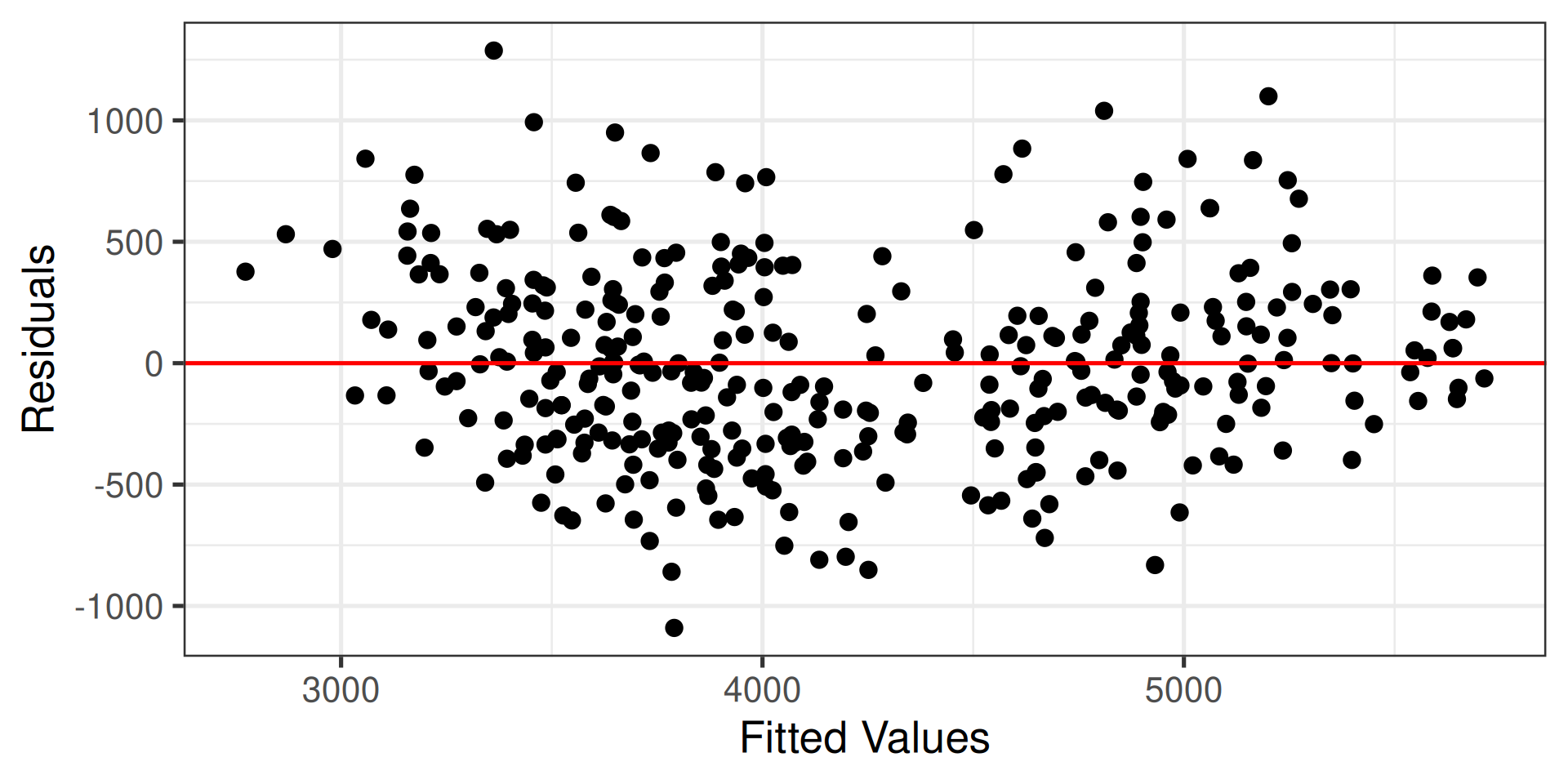
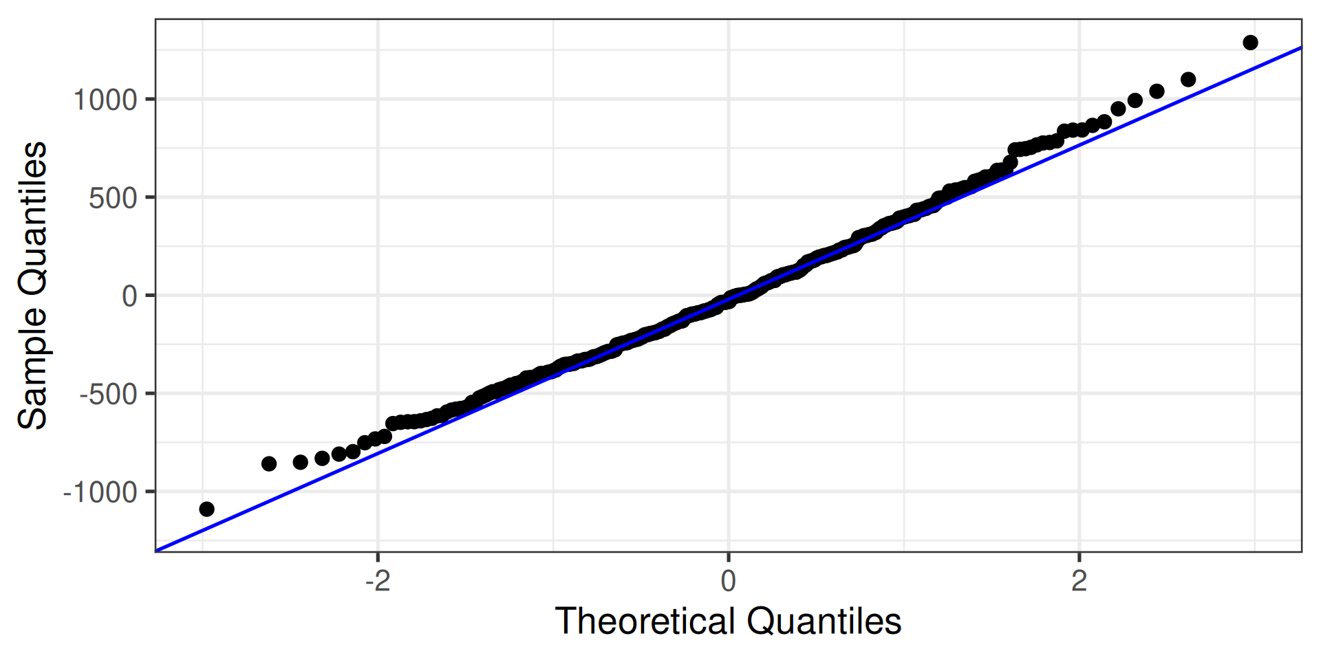
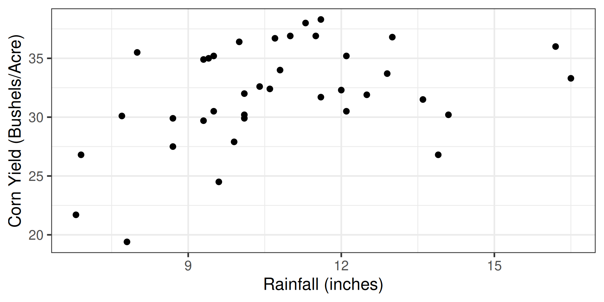
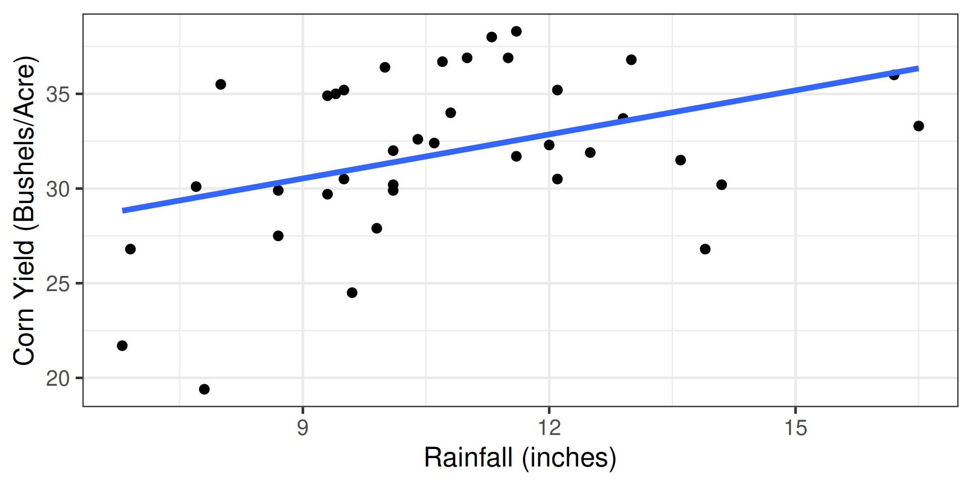
A team of agricultural researchers collected information on corn yield (Yield, measured in bushels per acre) as a function of annual rainfall (Rainfall, measured in inches):

\[ \widehat{\texttt{Yield}}_i = 23.55 + 0.78 \left( \texttt{Rainfall}_i \right) \]

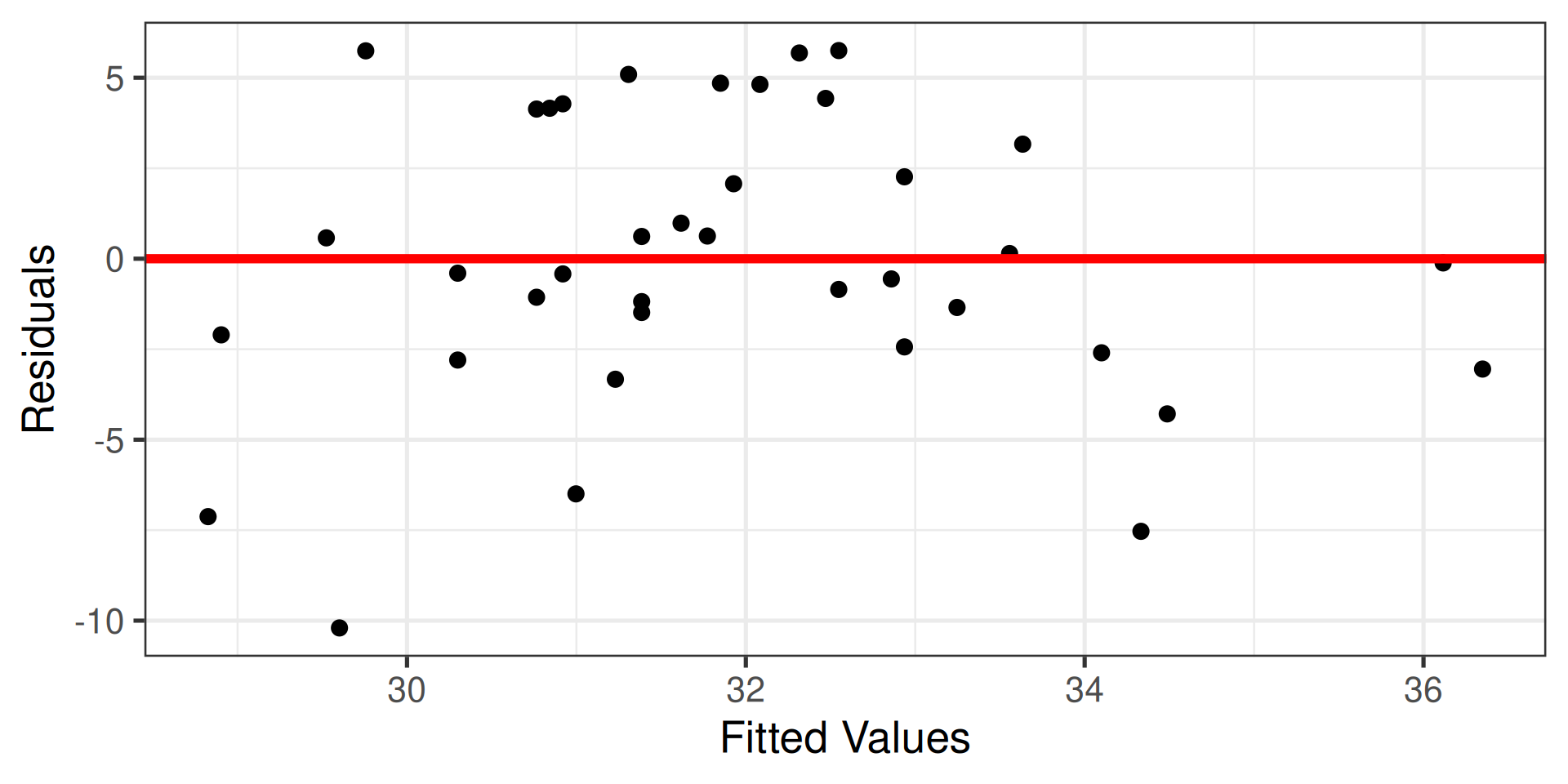
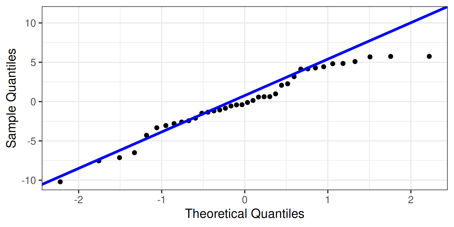
Example: rainfall and corn yield

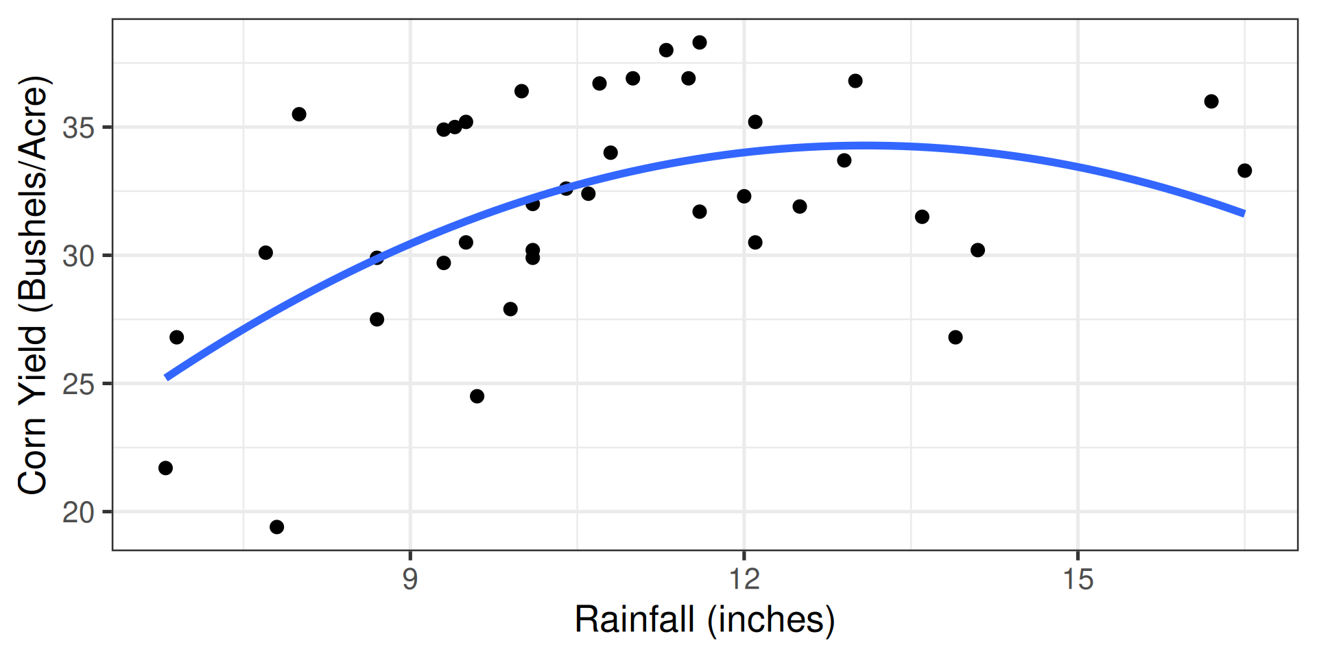
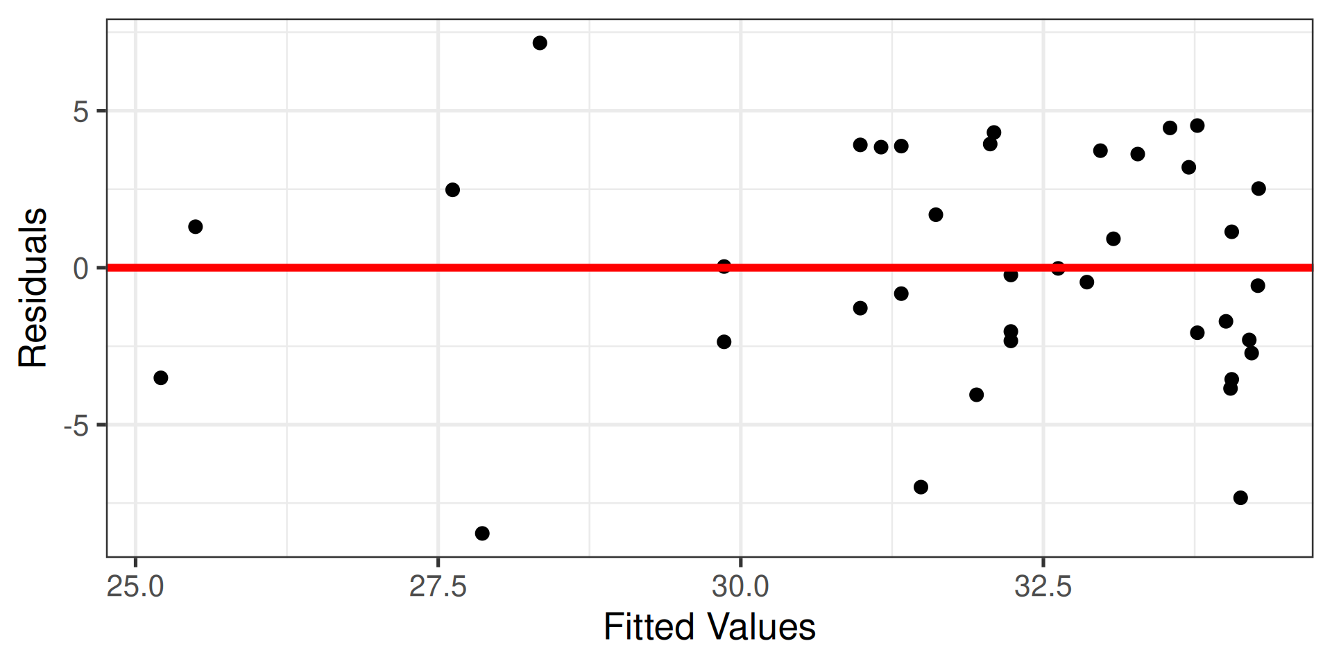
Increasing rain is associated with increasing yield to a point before this relationship levels off (or even reverses)!

\[ \widehat{\texttt{Yield}}_i = -5.01 + 6.00 \left( \texttt{Rainfall}_i \right) - 0.23 \left( \texttt{Rainfall}_i \right)^2 \]

Ex: fitting a quadratic model in R

corn_quad_lm <- lm(Yield ~ Rainfall + I(Rainfall^2), data = corn)
summary(corn_quad_lm)


Call:
lm(formula = Yield ~ Rainfall + I(Rainfall^2), data = corn)

Residuals:
    Min      1Q  Median      3Q     Max 
-8.4642 -2.3236 -0.1265  3.5151  7.1597 

Coefficients:
              Estimate Std. Error t value Pr(>|t|)   
(Intercept)   -5.01466   11.44158  -0.438  0.66387   
Rainfall       6.00428    2.03895   2.945  0.00571 **
I(Rainfall^2) -0.22936    0.08864  -2.588  0.01397 * 
---
Signif. codes:  0 '***' 0.001 '**' 0.01 '*' 0.05 '.' 0.1 ' ' 1

Residual standard error: 3.763 on 35 degrees of freedom
Multiple R-squared:  0.2967,    Adjusted R-squared:  0.2565 
F-statistic: 7.382 on 2 and 35 DF,  p-value: 0.002115

Final thoughts

Tip

When we add interactions or polynomial terms, keep the main effects and lower order terms in the model, whether or not they are statistically significant!!

\[\begin{align*} \mathbb{E}[Y_i | x_{i1}, x_{i2}] &= \beta_0 + \beta_1 x_{i1} + \beta_2x_{i2} + \beta_3 x_{i1}x_{i2} \\ \mathbb{E}[Y_i | x_{i}] &= \beta_0 + \beta_1 x_{i} + \beta_2 x_{i}^2 \end{align*}\]

Once these terms are added: effect of one variable in the model no longer captured by a single coefficient
Can improve the way our model fits the data and highlight important features about the relationships between variables
- Increased flexibility \(\implies\) increased model complexity \(\implies\) more nuanced interpretation