15-ANOVA and Nested F-tests
SDS 291
Prof. Baumer
October 27, 2025
Recall: hypotheses with MLR
- Setting just one \(\beta\) coefficient in the model to zero (or another constant)
- Results of the \(t\)-test are reported directly in the
summary()output!
- Results of the \(t\)-test are reported directly in the
- Setting a weighted sum of \(\beta\) coefficients in the model to zero
- Conduct the \(t\)-test “by hand”, taking care when finding the standard error for the linear combination of coefficients
- Setting multiple separate \(\beta\) coefficients equal to zero simultaneously
- Conduct an \(F\)-test for model comparison!
Example: Palmer penguins
Research Question
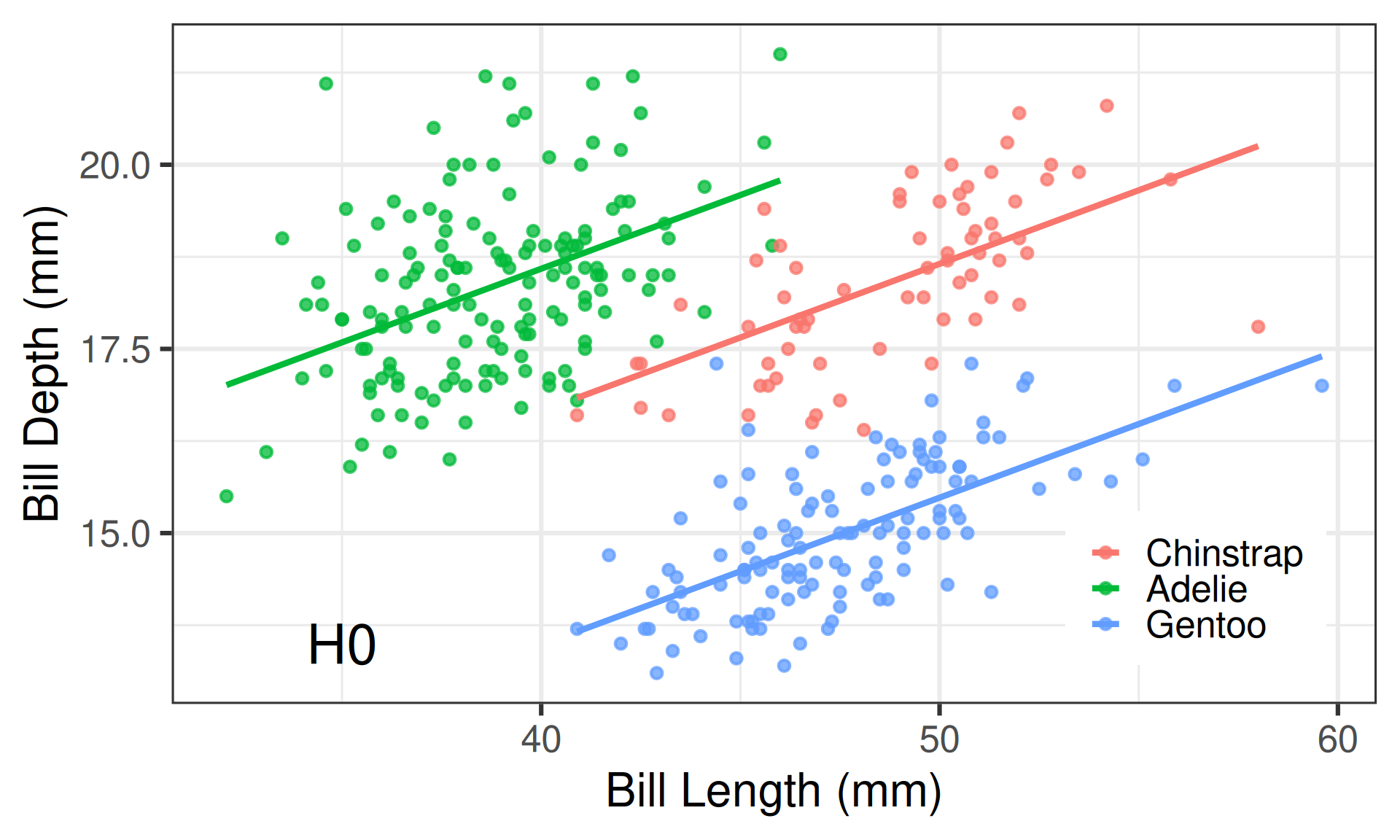
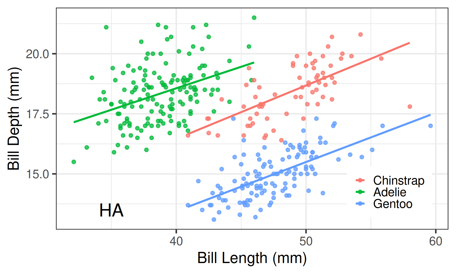
Does penguin species moderate/modify the relationship between bill length and bill depth?
\[\begin{gather*} {H_0:}\quad \mathbb{E}[\texttt{Depth}_i | x] = \beta_0 + \beta_1\texttt{Length}_i + \beta_2\texttt{Adelaide}_i + \beta_3\texttt{Gentoo}_i\\[-0.2em] vs.\\[-0.2em] {H_A:}\quad \mathbb{E}[\texttt{Depth}_i | x] = \beta_0 + \beta_1\texttt{Length}_i + \beta_2\texttt{Adelaide}_i + \beta_3\texttt{Gentoo}_i \\ \quad\quad + \beta_4\left(\texttt{Length}_i\right)\left(\texttt{Adelaide}_i\right) + \beta_5\left(\texttt{Length}_i\right)\left(\texttt{Gentoo}_i\right) \end{gather*}\]
🙈 p-values
Tip
Can’t just look at the individual \(p\)-values for the two interaction terms
Call:
lm(formula = bill_depth_mm ~ bill_length_mm * species, data = penguins)

Residuals:
    Min      1Q  Median      3Q     Max
-2.6574 -0.6675 -0.0524  0.5383  3.5032

Coefficients:
                             Estimate Std. Error t value Pr(>|t|)
(Intercept)                   7.56914    1.70983   4.427 1.29e-05 ***
bill_length_mm                0.22221    0.03493   6.361 6.55e-10 ***
speciesAdelie                 3.83998    2.05398   1.870   0.0624 .
speciesGentoo                -2.31813    2.16945  -1.069   0.2860
bill_length_mm:speciesAdelie -0.04338    0.04558  -0.952   0.3419
bill_length_mm:speciesGentoo -0.01737    0.04480  -0.388   0.6985
---
Signif. codes:  0 '***' 0.001 '**' 0.01 '*' 0.05 '.' 0.1 ' ' 1

Residual standard error: 0.9548 on 336 degrees of freedom
  (2 observations deleted due to missingness)
Multiple R-squared:  0.7697,    Adjusted R-squared:  0.7662
F-statistic: 224.5 on 5 and 336 DF,  p-value: < 2.2e-16
Recall: SST
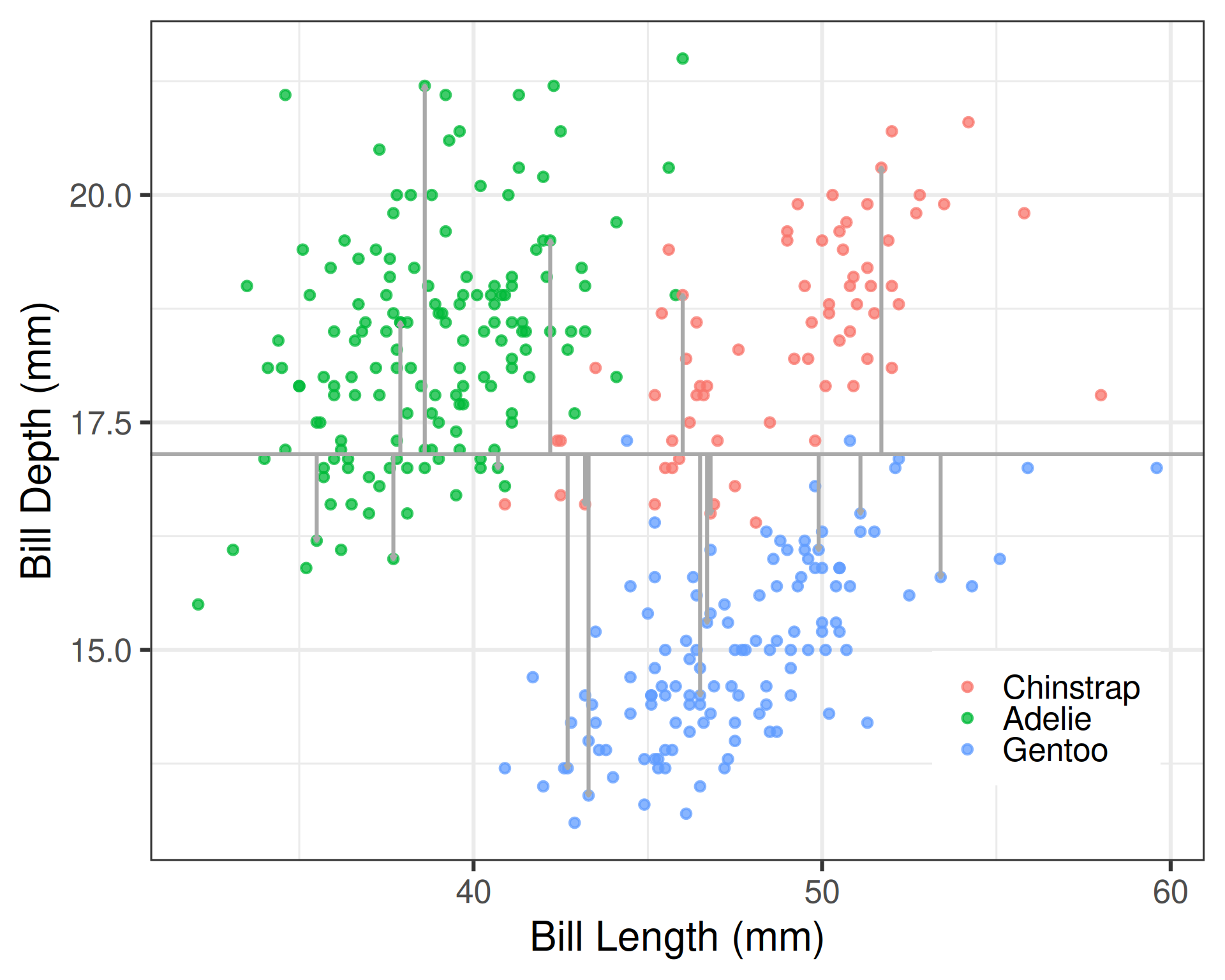
\[\begin{align*} SST &= \sum_{i=1}^{n}(y_i - \bar{y})^2\\[0.25em] df &= n - 1 \\[0.25em] MST &= \frac{SST}{n-1} \end{align*}\]
Recall: SSM
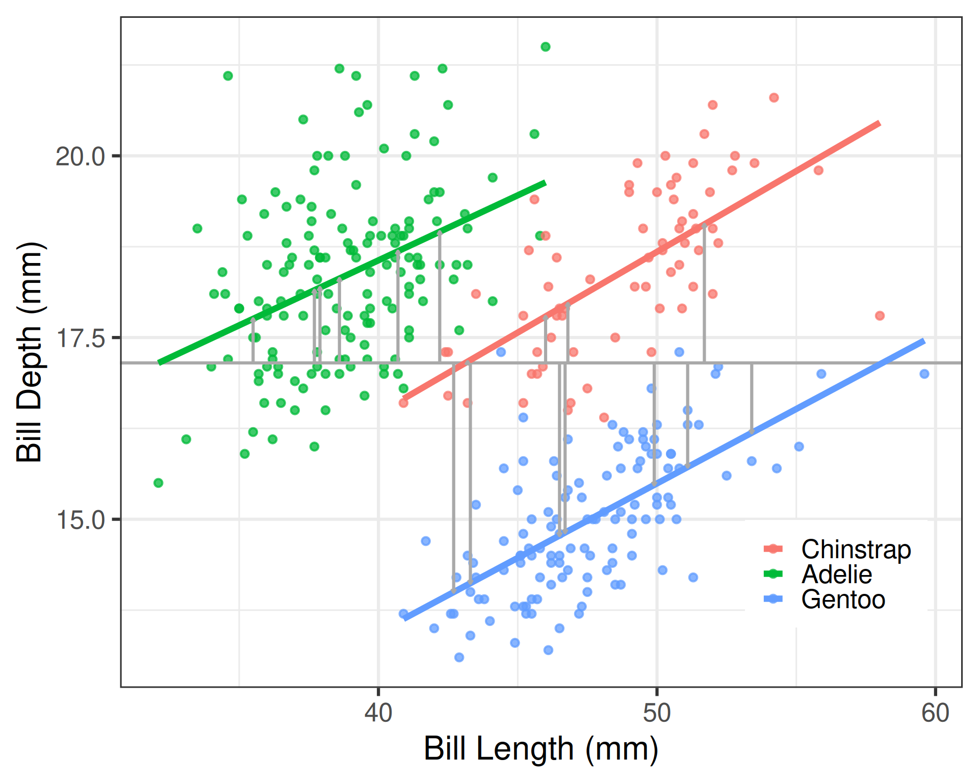
\[\begin{align*} SSM &= \sum_{i=1}^{n}(\widehat{y}_i - \bar{y})^2\\[0.25em] df &= k\\[0.25em] MSM &= \frac{SSM}{k} \end{align*}\]
Recall: SSE
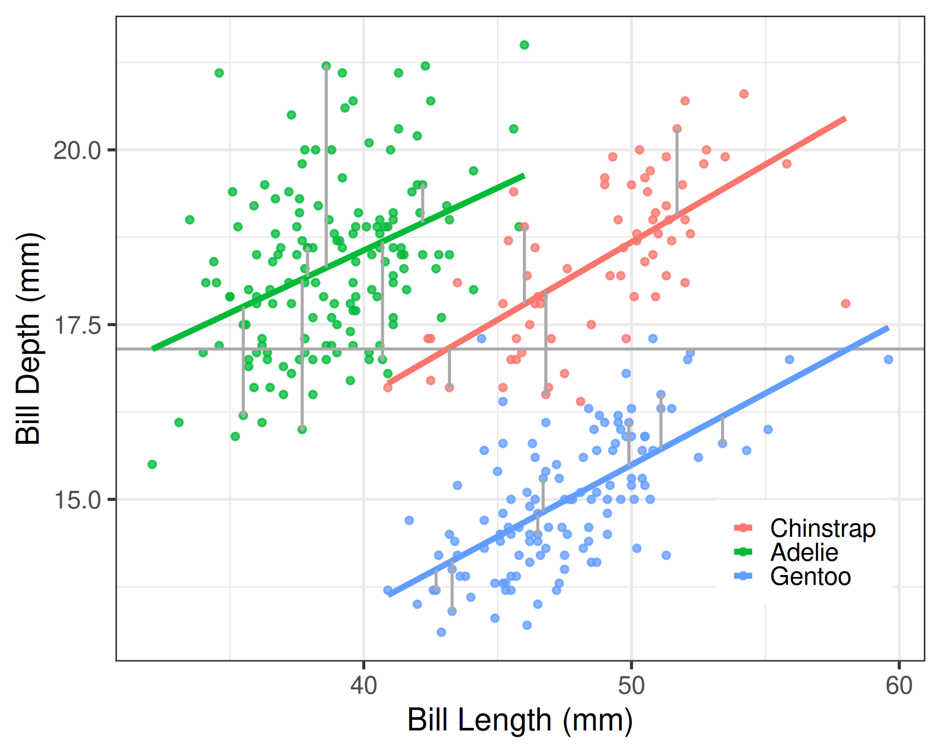
\[\begin{align*} SSE &= \sum_{i=1}^{n}(y_i - \widehat{y}_i)^2\\[0.25em] df &= n - k - 1\\[0.25em] MSE &= \frac{SSE}{n - k - 1} \end{align*}\]
Sum of squares decomposition in R
Sum of Squares Decomposition for SLR
Analysis of Variance Table

Response: bill_depth_mm
                Df  Sum Sq Mean Sq F value   Pr(>F)
bill_length_mm   1   73.47  73.473  19.884 1.12e-05 ***
Residuals      340 1256.36   3.695
---
Signif. codes:  0 '***' 0.001 '**' 0.01 '*' 0.05 '.' 0.1 ' ' 1
Sequential Sum of Squares Decomposition for MLR
Analysis of Variance Table

Response: bill_depth_mm
                        Df Sum Sq Mean Sq  F value Pr(>F)
bill_length_mm           1  73.47   73.47  80.5908 <2e-16 ***
species                  2 949.16  474.58 520.5569 <2e-16 ***
bill_length_mm:species   2   0.87    0.44   0.4785 0.6202
Residuals              336 306.32    0.91
---
Signif. codes:  0 '***' 0.001 '**' 0.01 '*' 0.05 '.' 0.1 ' ' 1
Note
- If you change the order of the variables in your
lm()model statement, you will end up with a different partition of the SSM - Overall SSM (the sum of all of these individual contributions) will always be the same, regardless of ordering!
Hypothesis testing with ANOVA
We can use the sum of squares decomposition to conduct two main flavors of hypothesis testing for (multiple) linear regression models:
- Overall F-Test: Are any of the predictor terms associated with the response?
- Nested F-Test: Do a particular subset of the predictor terms contribute meaningfully to the model?
Plot Twist!
Although your textbook presents them as two separate ideas, these two tests are actually the same thing! All \(F\)-tests are nested \(F\)-tests by design.
What do we mean by “nested”?

We have a “small” model and a “large” model, where the “small” model is completely contained in the “large” model!
Examples of nested models
- One Set of Nested Models
- Small: \(\mathbb{E}[Y] = \beta_0\)
- Large: \(\mathbb{E}[Y | x] = \beta_0 + \beta_1x_1 + \beta_2x_2 + \cdots + \beta_k x_k\)
- Another Set of Nested Models:
- Small: \(\mathbb{E}[Y| x_1] = \beta_0 + \beta_1 x_1\)
- Large: \(\mathbb{E}[Y | x_1, x_2] = \beta_0 + \beta_1x_1 + \beta_2x_2 + \beta_3 x_1x_2\)
- A Third Set of Nested Models:
- Small: \(\mathbb{E}[Y|x_1, x_2] = \beta_0 + \beta_c(x_1 + x_2) + \beta_3x_1x_2\)
- Large: \(\mathbb{E}[Y|x_1, x_2] = \beta_0 + \beta_1x_1 + \beta_2x_2 + \beta_3x_1x_2\)
How to nest models
In general, for models to be nested we:
- Should be able to obtain the small model by placing constraints on the large model (e.g., setting some slope terms to zero)
- Need to fit both models using the exact same data
Warning
This last condition is especially important when we have missing data in one or more of the predictor terms \(\implies\) filter out observations that have missing data in any of the variables in the full model before fitting any of the models of interest!
What’s so special about nested?
If (and only if) two linear regression models are nested in one another, then the model sums of squares (SSMs) for the two models are connected:
\[\begin{align*} \underbrace{SSM(x_1, x_2, x_3)}_{\substack{\text{variability explained}\\[0.25em] \text{by the full model}}} &= \underbrace{SSM(x_1, x_2)}_{\substack{\text{variability explained}\\[0.25em] \text{by the reduced model}}} + \underbrace{SSM(x_3 | x_1, x_2)}_{\substack{\text{additional variability explained} \\[0.25em] \text{by the extra term(s)}}} \end{align*}\]
The nested F-test
- Setup:
- full (large) model contains \(k\) predictor terms
- reduced (small) model contains \(k - p\) predictors
- Q: Do the additional \(p\) terms in the full model contribute meaningfully to the model?
- Formulate two competing hypotheses:
- \(H_0: \beta_j = 0\) for all \(p\) predictor terms being dropped from the full model
- \(H_A:\) \(\beta_j \neq 0\) for at least one of the \(p\) predictor terms being dropped from the full model
Construct a test statistic
\[\begin{align*} F &= \frac{ \left( \frac{SSM_\text{reduced} - SSM_\text{full}}{p} \right) }{\left( \frac{SSE_\text{full}}{n-k-1} \right) } \\ &= \frac{(SSE_\text{reduced} - SSE_\text{full})/p}{MSE_\text{full}} \end{align*}\]
- Statisticians have shown that…
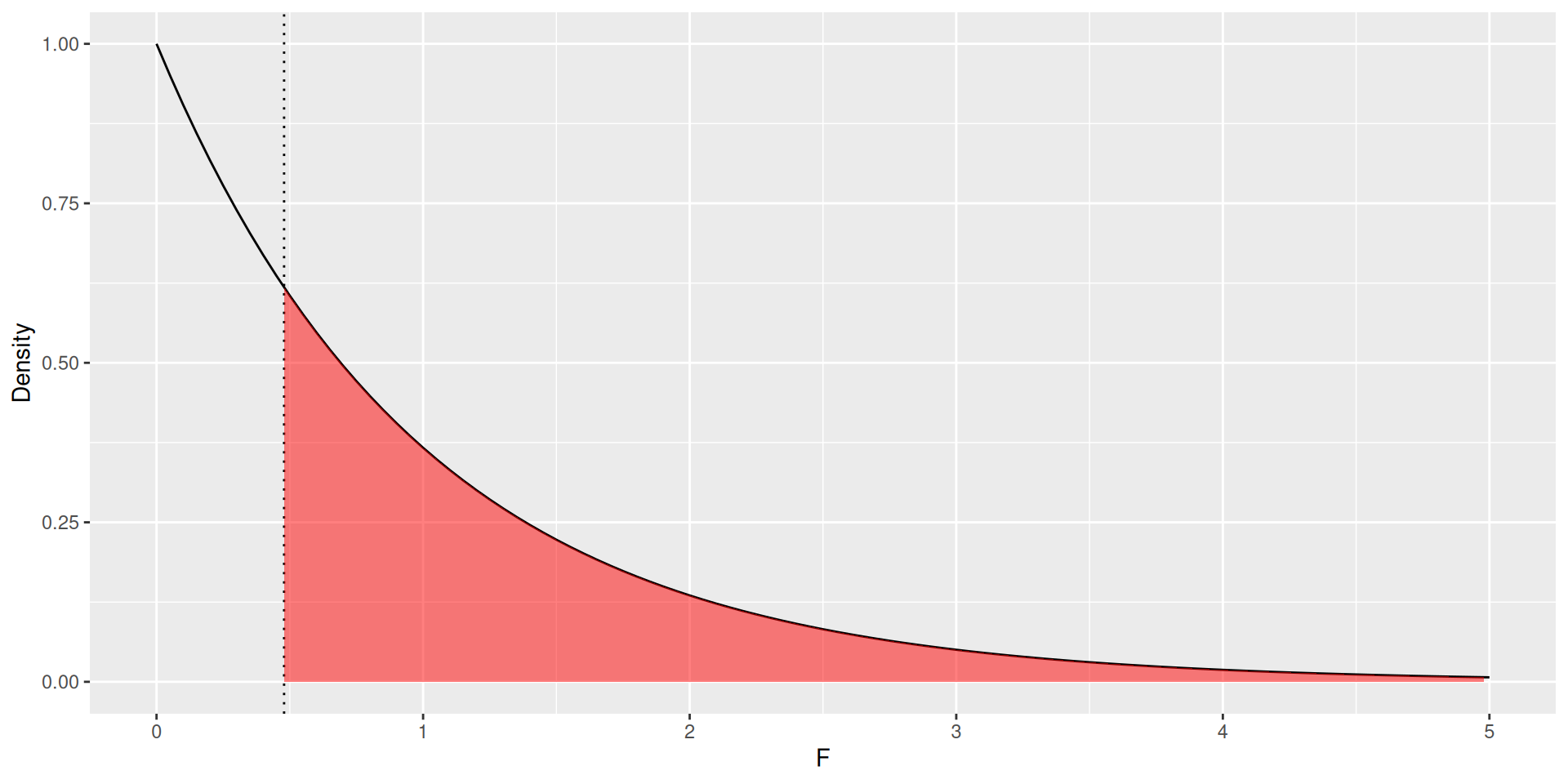
- sampling distribution of \(F\) is \(F(p, n-k-1)\)
The \(F(df_1, df_2)\) distribution
- Right-skewed distribution
- Shape is controlled by two parameters:
- numerator degrees of freedom, \(df_1\)
- denominator degrees of freedom, \(df_2\)
- Nested F-Test: \(df_1 = p\), \(df_2 = n - k - 1\)
- Use
pf(F, df1, df2, lower.tail = FALSE)
The nested \(F\)-test: 🐧
Conduct nested F-tests in R using anova(reduced, full):
# Removing all penguins with missing bill length, bill depth, or species
penguins_cc <- penguins |>
  drop_na(contains("bill_"), species)

# Fitting the full and reduced models
interact_lm <- lm(bill_depth_mm ~ bill_length_mm * species, data = penguins_cc)
parallel_lm <- update(interact_lm, . ~ . - bill_length_mm:species)

# Conducting the nested F-test
anova(parallel_lm, interact_lm)
Analysis of Variance Table
Model 1: bill_depth_mm ~ bill_length_mm + species
Model 2: bill_depth_mm ~ bill_length_mm * species
Res.Df RSS Df Sum of Sq F Pr(>F)
1 338 307.20
2 336 306.32 2 0.87243 0.4785 0.6202Decoding the anova() output
Analysis of Variance Table

Model 1: bill_depth_mm ~ bill_length_mm + species
Model 2: bill_depth_mm ~ bill_length_mm * species
  Res.Df    RSS Df Sum of Sq      F Pr(>F)
1    338 307.20
2 336 306.32 2 0.87243 0.4785 0.6202- Reduced Model: \(df = 338 = 342 - (3 + 1), SSE = 307.20\)
- Full Model: \(df = 336 = 342 - (5 + 1), SSE = 306.32\)
- Extra Sum of Squares: \(SSE_\text{reduced} - SSE_\text{full} = 307.20 - 306.32 = 0.87243\)
- # Constraints Tested: \(df_\text{reduced} - df_\text{full} = 338 - 336 = 2\)
- F-statistic: \(\frac{(\text{Extra Sum of Squares})/\# \text{ constraints}}{SSE_\text{full}/df_\text{full}} = \frac{0.87243/2}{306.32/336} = 0.4785\)
There is only one test!
Example: Palmer penguins
Research Question
Does penguin species moderate the relationship between bill length and bill depth?
Conclusion
We fail to reject the null hypothesis and conclude that the relationship between bill length and bill depth does not significantly differ across the three penguin species (\(p = 0.62\)).
Overall \(F\)-test
Research Question
Are any of penguin species, penguin bill length, or their interaction useful in modeling the bill depth of Antarctic penguins?
Call:
lm(formula = bill_depth_mm ~ bill_length_mm * species, data = penguins_cc)

Residuals:
    Min      1Q  Median      3Q     Max
-2.6574 -0.6675 -0.0524  0.5383  3.5032

Coefficients:
                             Estimate Std. Error t value Pr(>|t|)
(Intercept)                   7.56914    1.70983   4.427 1.29e-05 ***
bill_length_mm                0.22221    0.03493   6.361 6.55e-10 ***
speciesAdelie                 3.83998    2.05398   1.870   0.0624 .
speciesGentoo                -2.31813    2.16945  -1.069   0.2860
bill_length_mm:speciesAdelie -0.04338    0.04558  -0.952   0.3419
bill_length_mm:speciesGentoo -0.01737    0.04480  -0.388   0.6985
---
Signif. codes:  0 '***' 0.001 '**' 0.01 '*' 0.05 '.' 0.1 ' ' 1

Residual standard error: 0.9548 on 336 degrees of freedom
Multiple R-squared:  0.7697,    Adjusted R-squared:  0.7662
F-statistic: 224.5 on 5 and 336 DF, p-value: < 2.2e-16- \(F = 224.5\), within \(F(df_1=5, df_2=336)\)
Conclusion
We have very strong evidence that at least one of these terms is necessary (\(p < 0.0001\)).
Nested \(F\)-test
Analysis of Variance Table

Model 1: bill_depth_mm ~ 1
Model 2: bill_depth_mm ~ bill_length_mm * species
  Res.Df     RSS Df Sum of Sq      F    Pr(>F)
1    341 1329.83
2    336  306.32  5    1023.5 224.53 < 2.2e-16 ***
---
Signif. codes: 0 '***' 0.001 '**' 0.01 '*' 0.05 '.' 0.1 ' ' 1- \(F = 224.5\), within \(F(df_1=5, df_2=336)\)
Conclusion
We have very strong evidence that at least one of these terms is useful (\(p < 0.0001\)).
Digging deeper
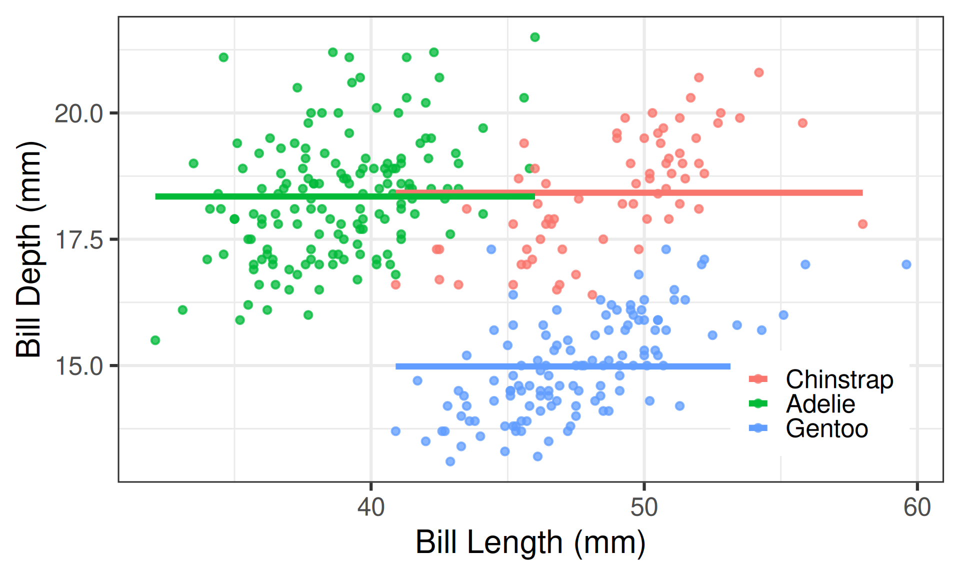
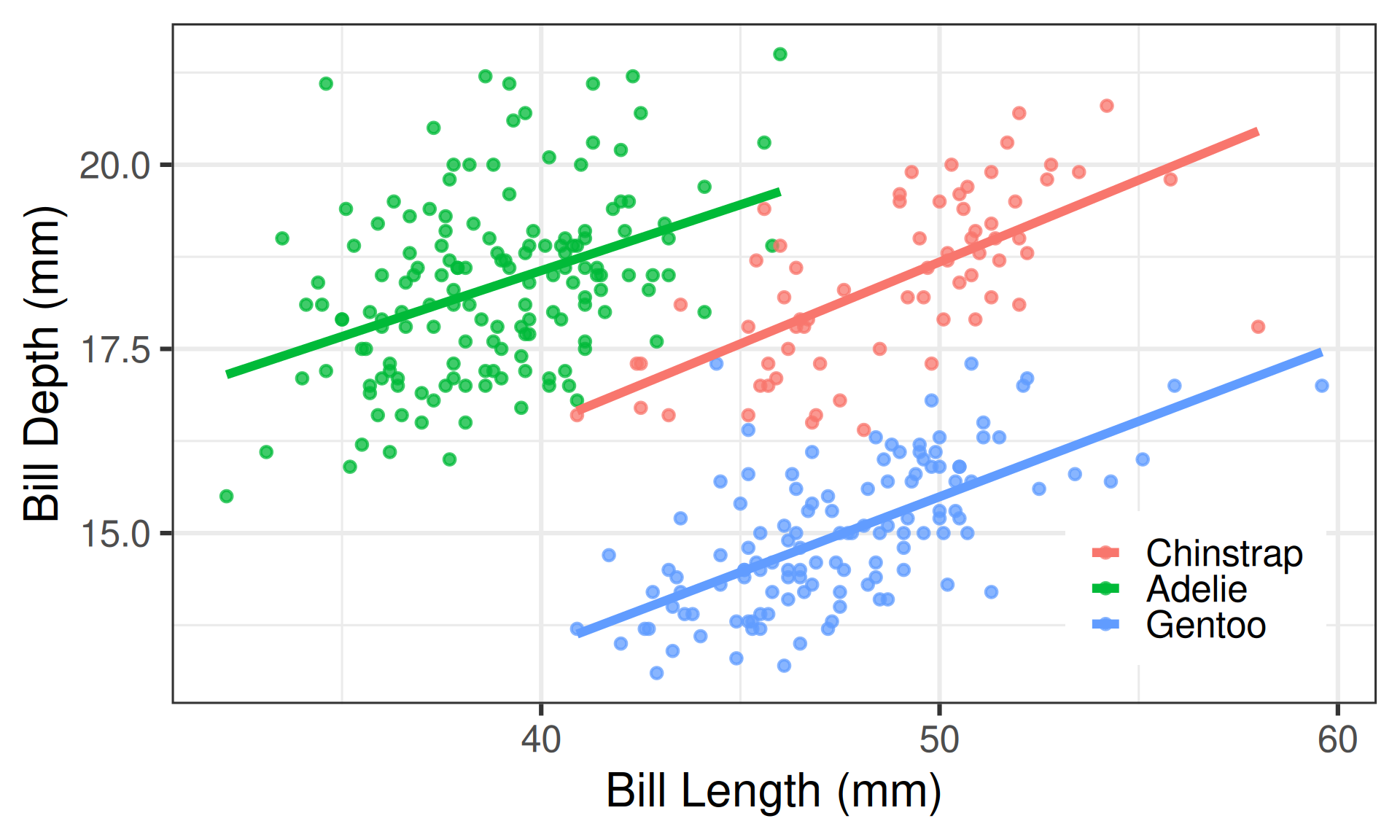
Research Question
Does bill length provide additional necessary information about the mean bill depth of penguins after first accounting for penguin species?
\[\begin{gather*} H_0: \quad \mathbb{E}[\texttt{Depth}_i | x] = \beta_0 + \beta_1\texttt{Adelie}_i + \beta_2\texttt{Gentoo}_i\\ vs.\\ H_A: \quad \mathbb{E}[\texttt{Depth}_i | x] = \beta_0 + \beta_1\texttt{Length}_i + \beta_2\texttt{Adelie}_i + \beta_3\texttt{Gentoo}_i \end{gather*}\]
\(F\)-test to \(t\)-test
Analysis of Variance Table

Model 1: bill_depth_mm ~ species
Model 2: bill_depth_mm ~ bill_length_mm + species
  Res.Df    RSS Df Sum of Sq      F    Pr(>F)
1    339 425.87
2    338 307.20  1    118.67 130.57 < 2.2e-16 ***
---
Signif. codes:  0 '***' 0.001 '**' 0.01 '*' 0.05 '.' 0.1 ' ' 1
Conclusion
There is strong evidence that bill length is associated with bill depth, even after accounting for penguin species (\(p < 0.0001\)).
Connecting the \(F\)-test
Tip
The nested \(F\)-test for testing \(k = 1\) predictor terms will always yield the exact same results as the \(t\)-test for that individual term!
                 Estimate Std. Error   t value     Pr(>|t|)
(Intercept)     8.6589862 0.86206892  10.04442 6.039045e-21
bill_length_mm  0.1998943 0.01749365  11.42668 8.661124e-26
speciesAdelie   1.9331943 0.22416005   8.62417 2.545386e-16
speciesGentoo  -3.1728258 0.14592926 -21.74222 3.473444e-66
Analysis of Variance Table
Model 1: bill_depth_mm ~ species
Model 2: bill_depth_mm ~ bill_length_mm + species
Res.Df RSS Df Sum of Sq F Pr(>F)
1 339 425.87
2 338 307.20 1 118.67 130.57 < 2.2e-16 ***
---
Signif. codes: 0 '***' 0.001 '**' 0.01 '*' 0.05 '.' 0.1 ' ' 1- \(F=130.57 = t^2 = 11.427^2\)!
- \(\rightarrow\) The \(p\)-values are also the same!
Some cautionary notes
- \(F\)-tests, like \(t\)-tests and \(t\)-based confidence intervals, are only valid if our regression conditions hold for the full (large) model
- Always check linearity, independence, Normality, and equal variance before interpreting or using your model for inference
- Can’t use hypothesis testing to help us choose between different possible transformations \(\implies\) use trial-and-error, along with your best judgement
- R/your computer is powerful, but only to a point! So always do your due diligence before turning to R:
- Determine what hypotheses you are interested in testing or what models you are comparing
- Make sure you know how to test/compare them appropriately

SDS 291