16-Linear Combinations of Coefficients
SDS 291
October 29, 2025
Inference for linear combinations
Many research questions of interest correspond not to a single coefficient in the model, but rather to a linear combination of coefficients: \[ \gamma = c_0\beta_0 + c_1\beta_1 + \cdots + c_k \beta_k, \] where \(c_0, \ldots, c_k\) are known constants, some of which may be zero.
These combinations allow us to:
- Compare non-reference levels of a categorical variable!
- Test slopes (e.g., in interaction or polynomial models) that involve multiple coefficients!
- Build hypothesis tests and confidence intervals for population means!
Recall interaction model 🐧
Research Question
Is there a relationship between the bill length and bill depth of Adelie penguins?
- No longer captured by just one parameter!
- \(\beta_1\): slope for bill length in the reference level (Chinstrap penguins)
- \(\beta_4\): adjustment to the slope for being in a non-reference level (Adelie penguins)
- \(\beta_1 + \beta_4\): slope for bill length among Adelie penguins
Our interaction model 🐧
Call:
lm(formula = bill_depth_mm ~ bill_length_mm * species, data = penguins)

Residuals:
    Min      1Q  Median      3Q     Max
-2.6574 -0.6675 -0.0524  0.5383  3.5032

Coefficients:
                             Estimate Std. Error t value Pr(>|t|)
(Intercept)                   7.56914    1.70983   4.427 1.29e-05 ***
bill_length_mm                0.22221    0.03493   6.361 6.55e-10 ***
speciesAdelie                 3.83998    2.05398   1.870   0.0624 .
speciesGentoo                -2.31813    2.16945  -1.069   0.2860
bill_length_mm:speciesAdelie -0.04338    0.04558  -0.952   0.3419
bill_length_mm:speciesGentoo -0.01737    0.04480  -0.388   0.6985
---
Signif. codes:  0 '***' 0.001 '**' 0.01 '*' 0.05 '.' 0.1 ' ' 1

Residual standard error: 0.9548 on 336 degrees of freedom
  (2 observations deleted due to missingness)
Multiple R-squared:  0.7697,    Adjusted R-squared:  0.7662
F-statistic: 224.5 on 5 and 336 DF,  p-value: < 2.2e-16
What about just Adelie 🐧?
- Formulate competing hypotheses: \[ H_0: \ \beta_1 + \beta_4 = 0 \quad \text{vs.}\quad H_A: \beta_1 + \beta_4 \neq 0. \]
- Determine a test statistic: \[ g = \widehat{\beta}_1 + \widehat{\beta}_4 = 0.222 + (-0.043) = 0.179 \]
- Estimate standard error: \[ SE(g) = SE(\widehat{\beta}_1 + \widehat{\beta}_4) = \sqrt{Var(\widehat{\beta}_1 + \widehat{\beta}_4)} \]
What is \(Var(\widehat{\beta}_1 + \widehat{\beta}_4)\)?
- Using standard variance propagation results
- Since \(\widehat{\beta}_1\) and \(\widehat{\beta}_4\) are r.v.’s: \[\begin{align*} \widehat{Var}(\widehat{\beta}_1 + \widehat{\beta}_4) &= \widehat{Var}(\widehat{\beta}_1) + \widehat{Var}(\widehat{\beta}_4) + 2 \cdot \widehat{Cov}(\widehat{\beta}_1, \widehat{\beta}_4) \\ \end{align*}\]
- What is covariance?
Variance-covariance matrix
- For an additive multiple regression model with two explanatory variables, \(\widehat{y}_i = \widehat{\beta}_0 + \widehat{\beta}_1 x_{i1} + \widehat{\beta}_2x_{i2}\),
\[\begin{equation*} \left[\begin{array}{c c c} Var(\widehat{\beta}_0) & Cov(\widehat{\beta}_0, \widehat{\beta}_1) & Cov(\widehat{\beta}_0, \widehat{\beta}_2)\\[0.4em] Cov(\widehat{\beta}_1, \widehat{\beta}_0) & Var(\widehat{\beta}_1) & Cov(\widehat{\beta}_1, \widehat{\beta}_2) \\[0.4em] Cov(\widehat{\beta}_2, \widehat{\beta}_0) & Cov(\widehat{\beta}_2, \widehat{\beta}_1) & Var(\widehat{\beta}_2) \end{array}\right] \end{equation*}\]
- Covariance: scaled version of the correlation that measures the (linear) relationship between the estimated coefficients
- Accessed using the R command
vcov()
Matrix for the interaction model
                             (Intercept) bill_length_mm speciesAdelie
(Intercept)                   2.92352319   -0.059592223   -2.92352319
bill_length_mm               -0.05959222    0.001220306    0.05959222
speciesAdelie                -2.92352319    0.059592223    4.21884345
speciesGentoo                -2.92352319    0.059592223    2.92352319
bill_length_mm:speciesAdelie  0.05959222   -0.001220306   -0.09282853
bill_length_mm:speciesGentoo  0.05959222   -0.001220306   -0.05959222
                             speciesGentoo bill_length_mm:speciesAdelie
(Intercept)                    -2.92352319                  0.059592223
bill_length_mm                  0.05959222                 -0.001220306
speciesAdelie                   2.92352319                 -0.092828532
speciesGentoo                   4.70649206                 -0.059592223
bill_length_mm:speciesAdelie   -0.05959222                  0.002077102
bill_length_mm:speciesGentoo   -0.09696853                  0.001220306
                             bill_length_mm:speciesGentoo
(Intercept)                                   0.059592223
bill_length_mm                               -0.001220306
speciesAdelie                                -0.059592223
speciesGentoo                                -0.096968528
bill_length_mm:speciesAdelie                  0.001220306
bill_length_mm:speciesGentoo                  0.002007095
The numbers we need
                             bill_length_mm bill_length_mm:speciesAdelie
bill_length_mm                  0.001220306                 -0.001220306
bill_length_mm:speciesAdelie   -0.001220306                  0.002077102
\[ SE(g) = \widehat{Var}(\widehat{\beta}_1) + \widehat{Var}(\widehat{\beta}_4) + 2 \cdot \widehat{Cov}(\widehat{\beta}_1, \widehat{\beta}_4) \]
Set up hypothesis test
- Formulate competing hypotheses: \[\begin{equation*} H_0: \ \beta_1 + \beta_4 = 0 \quad \text{vs.}\quad H_A: \beta_1 + \beta_4 \neq 0 \end{equation*}\]
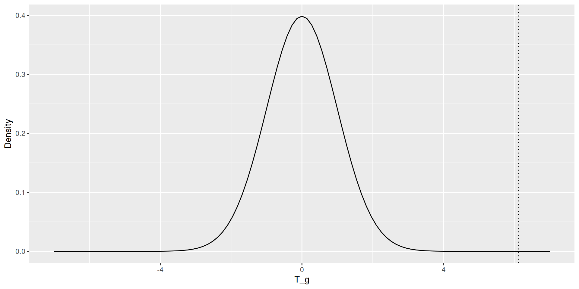
- Determine a test statistic: \[ T = \frac{(\widehat{\beta}_1 + \widehat{\beta}_4) - 0}{\widehat{SE}(\widehat{\beta}_1 + \widehat{\beta}_4)} = \frac{g}{SE(g)} \equiv \frac{0.179}{0.0293} = 6.110 \]
Ex: bill length and depth for Adelie 🐧
- Determine the null distribution: \(t_{n - k - 1} \equiv t_{336}\)
- Compare the test statistic to the null distribution: \[p = 2 \times \Pr(T > 6.110)\]
There is only one test!
Ex: CI for Adelie penguins
Research Question
What is a range of plausible values for the relationship between bill length and bill depth in Adelie penguins?
\[\begin{align*} (\widehat{\beta}_1 + \widehat{\beta}_4) \pm t^* \cdot \widehat{SE}(\widehat{\beta}_1 + \widehat{\beta}_4) &= g \pm t^* \cdot SE(g) \\ &= 0.179 \pm (1.97)(0.0293) \\ &= 0.179 \pm 0.058\\ &= (0.121, 0.236) \end{align*}\]
Final conclusions
Among Adelie penguins, we estimate that a one mm increase in bill length is associated with a 0.179 mm increase in mean bill depth; this relationship is statistically significant at the \(\alpha = 0.05\) level (\(p < 0.001\); 95% CI: 0.121, 0.236).
In other words, we reject the null hypothesis that there is no relationship between bill length and bill depth among Adelie penguins.

SDS 291