17-Influential Points
SDS 291
Prof. Baumer
November 3, 2025
Unusual points
Note
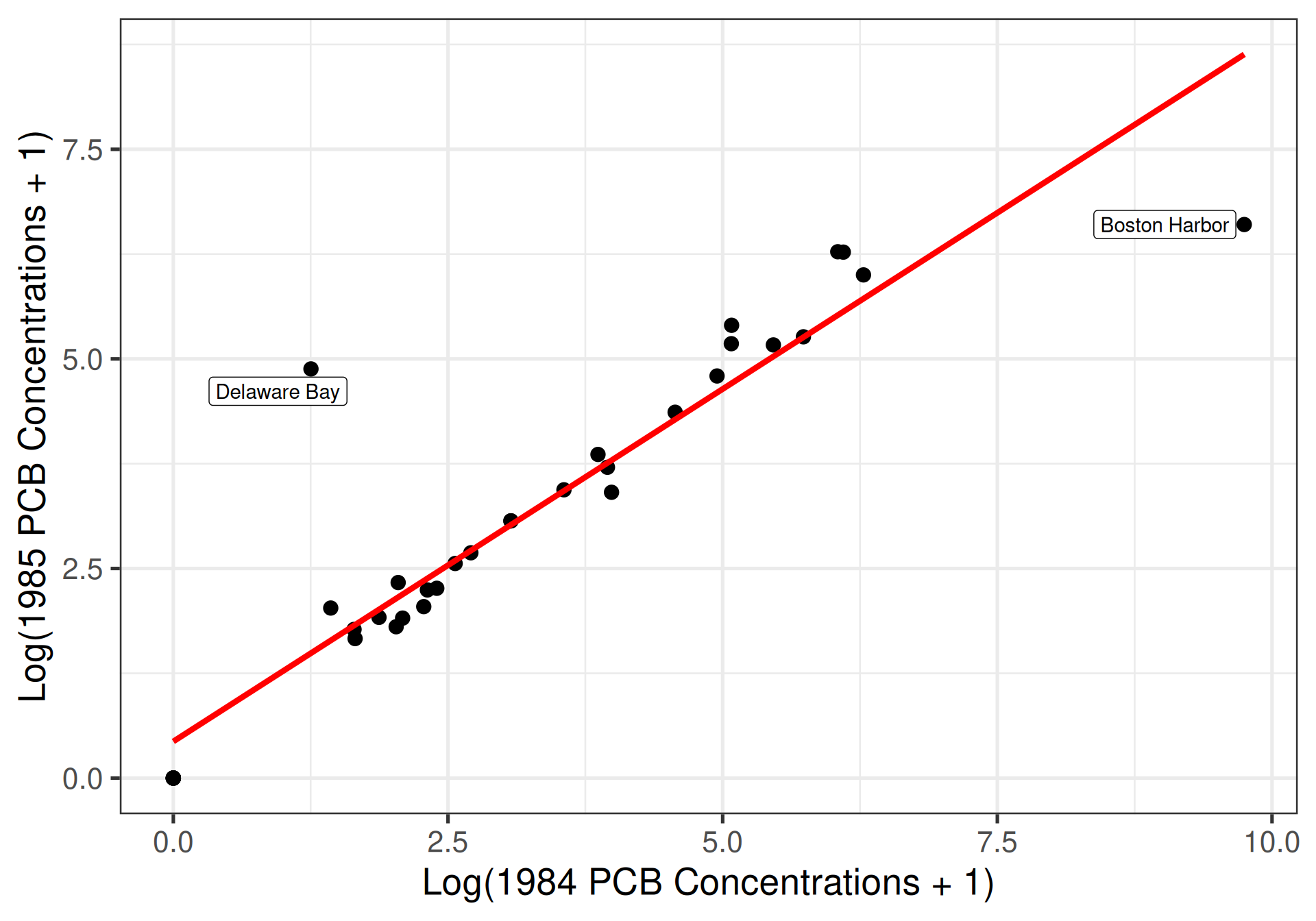
How do we do due diligence to make sure a small number of points don’t have outsized influence on our fitted regression model/conclusions?

Outliers
When is it OK to remove outliers?
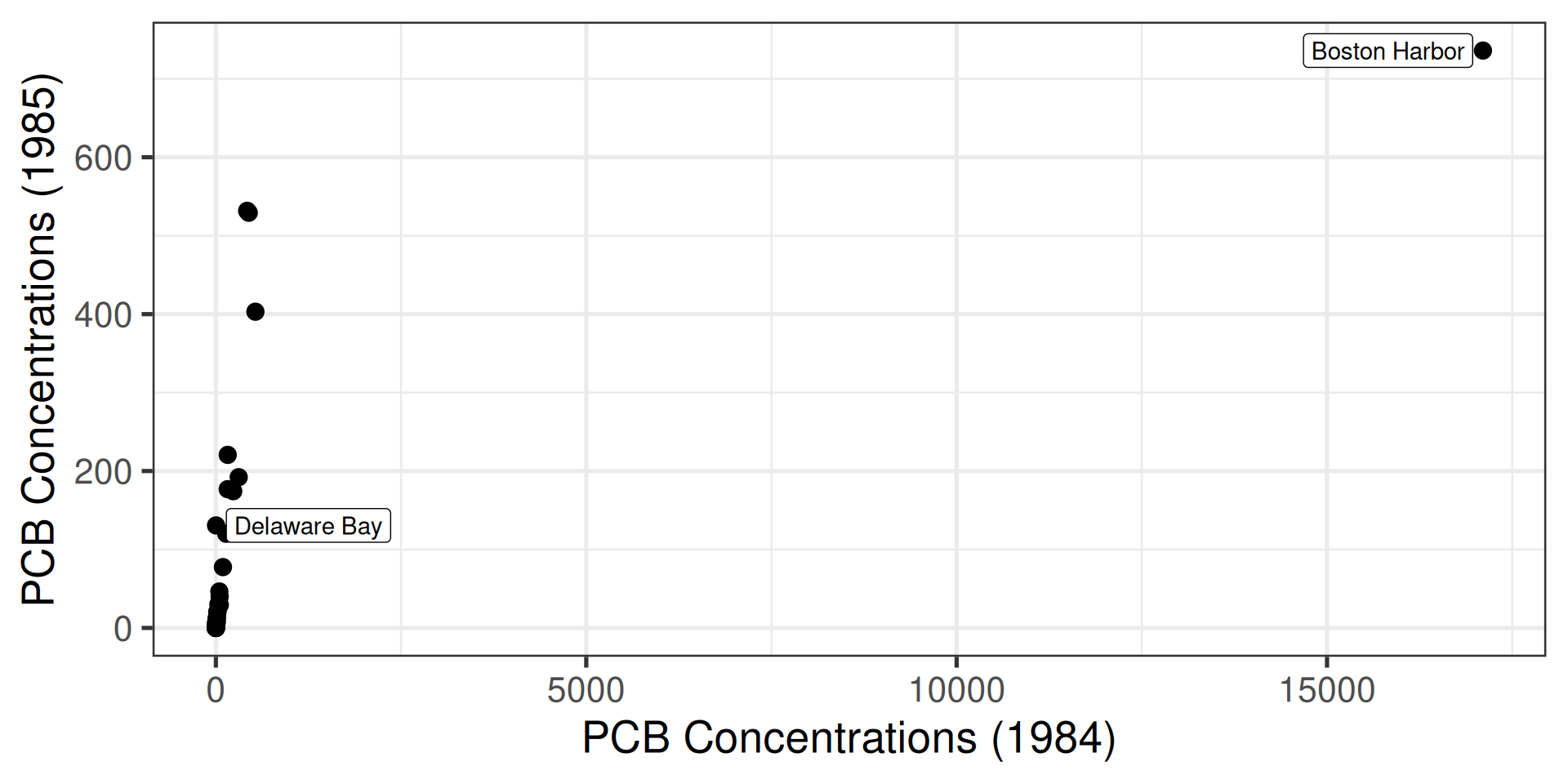
Some outliers affect slopes
Note effect of removing Boston Harbor
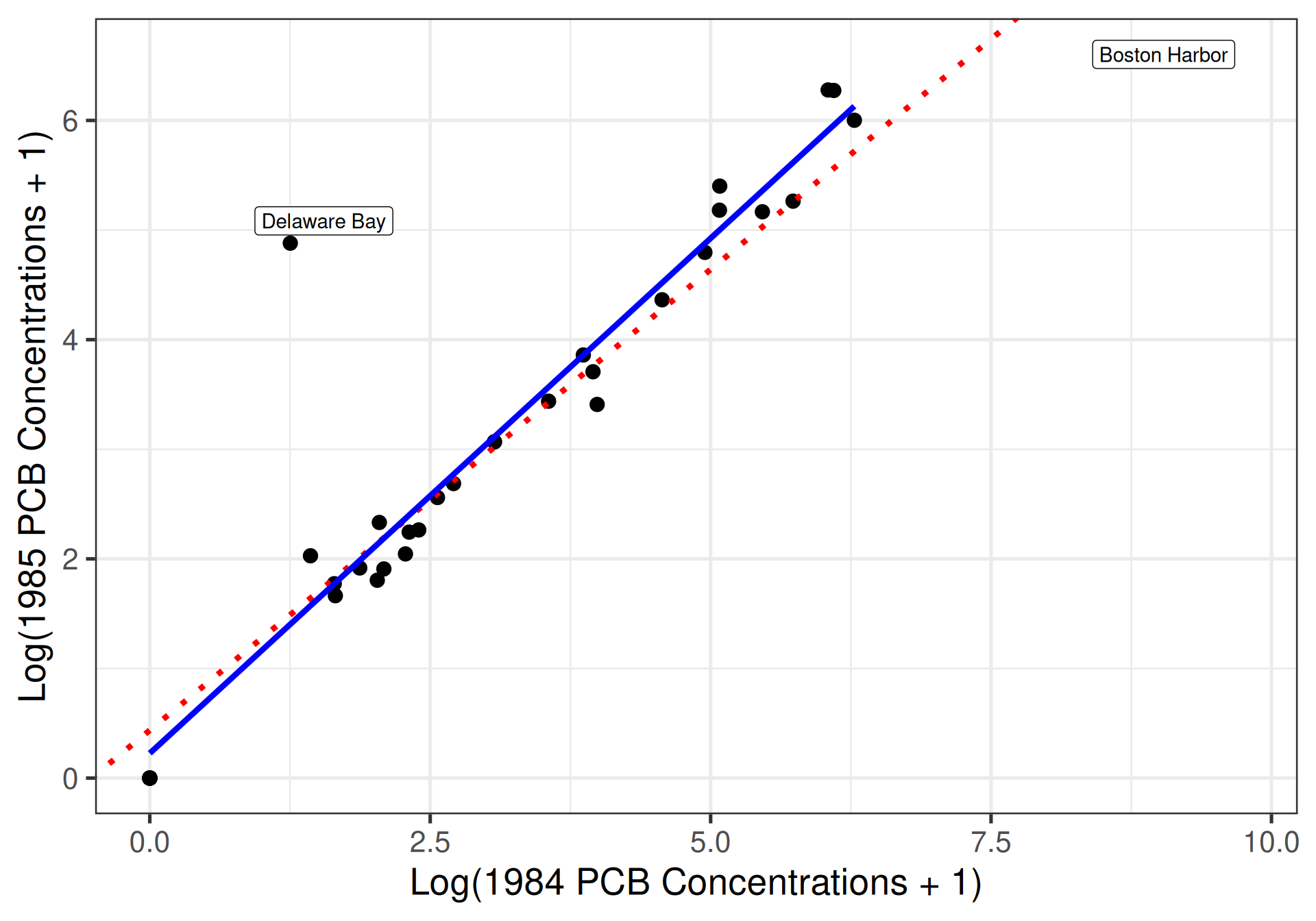
Note
How large is large enough to be misleading? And how else might we detect these sorts of influential points when visualization is challenging?
Diagnostic detectives
Influence of an individual observation depends on:
- Leverage: how extreme the value of (at least one of) its explanatory variables is
- Standardized/studentized residuals: how extreme (unusually large) the residual error is
Cook’s distance: Combine these two characteristics into one overall measure of case influence
Influential obs. are not like the others
Answer(s) to our question(s) of interest might change depending on whether or not we include them when fitting the model…
- Potential data quality issue or data entry error
- May be the result of random variation in the data
- May be the result of undersampling part of the population
- May belong to a different population than rest of the data
- May indicate something scientifically interesting
In any event, influential points are worth investigating further!
Investigative toolkit
Tools (case influence statistics) to investigate and identify influential observations through the augment() function:
.hat: leverage.std.resid: standardized residual.cooksd: Cook’s distance
# A tibble: 6 × 8
  `log(pcb85 + 1)` `log(pcb84 + 1)` .fitted   .resid   .hat .sigma    .cooksd
             <dbl>            <dbl>   <dbl>    <dbl>  <dbl>  <dbl>      <dbl>
1             4.36             4.57    4.28  0.0869  0.0417  0.763 0.000302
2             3.41             3.99    3.79 -0.381   0.0333  0.760 0.00458
3             6.00             6.28    5.72  0.284   0.0868  0.762 0.00739
4             6.60             9.75    8.63 -2.03    0.271   0.645 1.86
5             5.26             5.73    5.26  0.00496 0.0691  0.763 0.00000173
6             5.40             5.08    4.71  0.692   0.0520  0.754 0.0245
# ℹ 1 more variable: .std.resid <dbl>
Clue #1: leverage
Distance between an individual observation’s predictor value(s) and the “average” such values in the entire data set
- SLR: points that are a large distance away from the mean of the explanatory variable have high leverage \[ h_i = \frac{1}{n} + \frac{(x_i - \bar{x})^2}{\sum_{i=1}^{n}(x_i - \bar{x})^2} \]
- MLR: points that are far away from the main “cloud” of observations have high leverage
Tip
Points are flagged for further study if \(h_i > 2(k + 1)/n\)
Clue #2: standardized residuals
Scaled version of the residual error, \(e_i\), that captures the extremity of the \(y\)-value for the observation \[\begin{equation*} \text{stdres}_i = \frac{e_i - 0}{SD(e_i)} = \frac{y_i - \widehat{y}_i}{\widehat{\sigma}_\epsilon \sqrt{1 - h_i}}, \end{equation*}\] where \(\widehat{\sigma}_\epsilon\) is the RMSE. Will be large when:
- An observation has high leverage: \(h_i\) is large so that \(1 - h_i\), and thus the denominator is small
- An observation has a large residual: model does not predict \(y_i\) well, so that the numerator of \(\text{stdres}_i\) is large
Tip
Points are flagged for further study if \(stdres_i < -2\) or \(stdres_i > 2\), because they follow a \(t\)-distribution!
Clue #2a: studentized residuals
Observations with extreme residuals also increase the residual standard deviation, \(\widehat{\sigma}_\epsilon\), so unusual points can sometimes “hide” themselves
\[ \text{stdres}_i = \frac{y_i - \widehat{y}_i}{\widehat{\sigma}_\epsilon \sqrt{1 - h_i}}, \]
The studentized residual “uncovers” these points by using \(\widehat{\sigma}_{(-i)}\) instead, the RMSE for a model fit with the \(i\)th observation removed from the sample:
\[ \text{stures}_i = \frac{y_i - \widehat{y}_i}{\widehat{\sigma}_{(-i)}\sqrt{1 - h_i}}, \]
Tip
Can be found in R using rstudent() and are interpreted in the same way as standardized residuals
Clue #3: Cook’s distance
Captures how much the coefficient estimates change when a particular observation is omitted: \[ D_i = \left(\frac{\text{stdres}_i^2}{k + 1}\right)\left(\frac{h_i}{1 - h_i}\right), \] The Cook’s distance will be large when:
- An observation has high leverage, \(h_i\)
- An observation has a large standardized residual, \(\text{stdres}_i\)
Tip
Points are flagged for further study if \(D_i > 1\)
So… what next?
Investigate! What is it about these points that makes them so special?
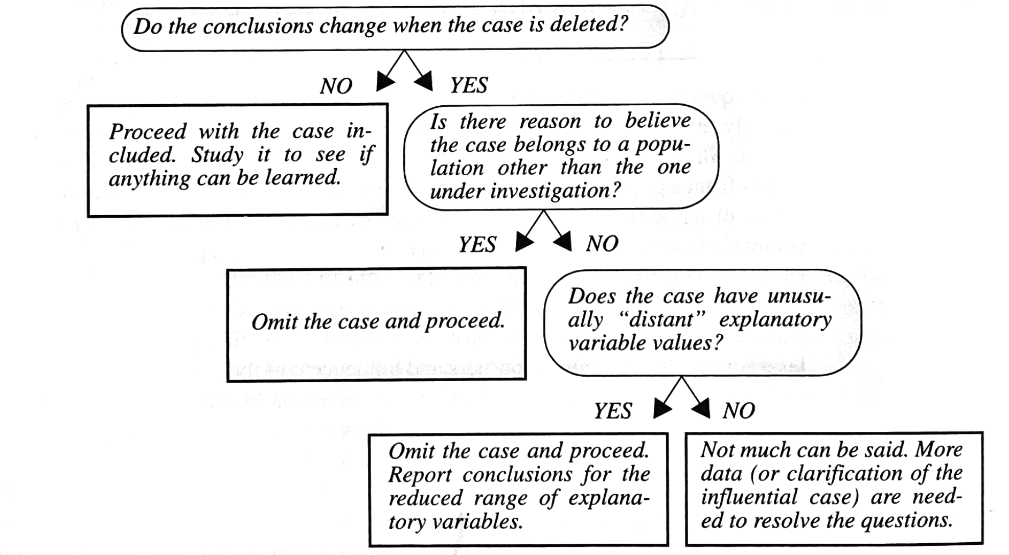
Typically only remove a data point if our final conclusions change substantially when we delete it (i.e., it has high \(D_i\)):
- Refit the model with the observation(s) removed
- Check conditions and conduct diagnostics on the new model
- Report the reason for removing the observation(s)
- Was it due to high leverage? Report how the removed case differs from the other data points and restrict conclusions to the reduced range of the explanatory variable(s)
- Are there potential errors in the data that are driving large standardized residuals?
- Does it belong to another population? Is it inherently different from the rest of the data points? (e.g., different type of ballot layout used)
To remove or not to remove?
- Exercise extreme caution when excluding data from a model
- Never remove a point just because your regression model looks “better” without it!
Where did our model come from?
- Modeling is not a static endeavor
- We often have a whole host of possible explanatory variables to choose from:
- water turbulence
- water temperature
- water depth
- presence of certain bacteria and fungi
- local climate regulations
- …
Note
How do we choose which combination or subset of explanatory variables is best?
Why not just include everything?
- Multicollinearity: more explanatory variables \(\Rightarrow\) more complex relationships between the explanatory variables
- Can increase our uncertainty in the estimated model and interfere with our ability to do inference
- Overfitting: more explanatory variables \(\nRightarrow\) more meaningful model
- Need to weigh the trade-off between explanatory power and complexity

SDS 291