18-Multicollinearity

SDS 291

Prof. Baumer

November 10, 2025

Where did our model come from?

  • Modeling is not a static endeavor
  • We often have a whole host of possible explanatory variables to choose from:
    • water turbulence
    • water temperature
    • water depth
    • presence of certain bacteria and fungi
    • local climate regulations

Note

How do we choose which combination or subset of explanatory variables is best?

Why not just include everything?

  • Multicollinearity: more explanatory variables \(\Rightarrow\) more complex relationships between the explanatory variables
    • Can increase our uncertainty in the estimated model and interfere with our ability to do inference
  • Overfitting: more explanatory variables \(\nRightarrow\) more meaningful model
    • Need to weigh the trade-off between explanatory power and complexity

Motivation #1: multicollinearity

Math test problem

Consider the following sequence of numbers:

\[ 2,\ 4, \ 8, \ 16, \ 32 \]

What rule generated this sequence?

  1. Ascending positive numbers
  2. Even numbers
  3. Powers of two
  • Yikes! Any of these rules could plausibly have generated the sequence!
  • This increases our uncertainty about the answer

What is multicollinearity?

A: the regression model equivalent of our multiple choice question:

  • One or more of the explanatory variables (answers) are strongly correlated
  • Exact collinearity: one variable is an exact linear function of the other variables
    • Ex: weight (in kg) \(= 2.2\ \times\) weight (in lbs)
    • Ex: an indicator for the \(k\)th level of a categorical variable would be collinear with the other \(k-1\) indicators
  • Approximate collinearity:
    • Ex: an individual’s height and the length of their inseam

Modeling height and weight

Suppose we want to model an individual’s weight and that we choose a model that includes their age, their height, and the inseam of their pants: \[ \mathbb{E}[\texttt{weight}_i | x] = \beta_0 + \beta_1 \left(\texttt{age}_i\right) + \beta_2\left({ \texttt{height}_i}\right) + \beta_3\left({\texttt{inseam}_i}\right) \]

The consequences of multicollinearity

Recall how we interpret slopes in an MLR model:

\(\beta_1\) captures the association between \(x_1\) and \(Y\) after controlling for (holding constant) all other variables in the model

As the correlation between explanatory variables increases:

  • The model has an increasingly difficult time parsing out which variables explain what portion of the variability in \(Y\)
  • Many different linear combinations of the explanatory variables will produce equally good fits, meaning our coefficient estimates can vary widely from sample to sample
  • Causes standard error, \(\widehat{SE}(\widehat{\beta}_1)\), to skyrocket
  • Geometric intuition: the plane gets “wobbly”!

Is it a problem?

Your turn!

Is multicollinearity necessarily a problem if:

  • Our goal is to classify or predict values of the outcome?
  • Our goal is to quantify and evaluate the strength of a relationship?

Consider the following:

  • fitted value, \(\widehat{y}\)
  • fitted coefficients, \(\widehat{\beta}\)
  • \(\widehat{SE}(\widehat{\beta})\)
  • model sum of squares, \(SSM\)
  • coefficient of determination, \(R^2\)
  • Which of these are important for which regression modeling goal?
  • Which are most impacted by multicollinearity?

Detecting multicollinearity (informal)

  1. Overall \(F\)-test for the model is significant, but none of the individual terms appear to be
  2. Coefficients have large standard errors and wide confidence intervals
  3. Coefficient has an opposite sign than expected
  4. Coefficients change substantially when another variable is added or removed
  5. Pairs of explanatory variables exhibit a strong linear relationship in a scatter plot matrix
  6. High pairwise correlation

Detecting multicollinearity (formal)

Variance Inflation Factor (VIF)

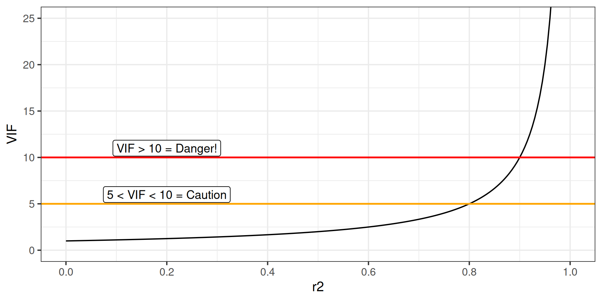
Captures the degree to which our uncertainty in \(\widehat{\beta}_j\) increases due to the other explanatory variables in the model: \[ \text{VIF}_j = \frac{1}{1 - R_j^2}, \] where \(R_j^2\) is the coefficient of determination for the linear regression of \(x_j\) on the other explanatory variables

  • Little collinearity (\(R_j^2 \approx 0\)): \(\text{VIF}_j \approx 1\)
  • Moderate collinearity (\(R_j^2 = 0.8\)): \(\text{VIF}_j = 5\)
  • Strong collinearity (\(R_j^2 = 0.9\)): \(\text{VIF}_j = 10\)

Tip

Variables with large VIFs are redundant with other explanatory variables in the model

Variance Inflation Factor (VIF)

Variance Inflation Factor (VIF)

Use vif() function in the car package

levi_jeans <- read_csv("https://raw.githubusercontent.com/kaitlyncook/data-sets/main/levis-jeans-1.csv")
# Calculating the VIF for height by hand
height_inseam_lm <- lm(height ~ inseam + age, data = levi_jeans)
height_inseam_lm |>
  glance() |>
  mutate(vif = 1 / (1 - r.squared)) |>
  select(r.squared, vif)
# A tibble: 1 × 2
  r.squared   vif
      <dbl> <dbl>
1     0.931  14.6
# Calculating the VIF for all variables using vif() in the car library
lm(weight ~ height + age + inseam, data = levi_jeans) |>
  car::vif()
  height      age   inseam 
14.57610  1.15165 14.82686