20-Odds and Odds Ratios

SDS 291

Prof. Baumer

November 12, 2025

Beyond linear regression

The type of response variable dictates the type of regression model that we build:

• Continuous response \(Y\) with Normally distributed errors \(\iff\) linear regression model \[ \text{observed data} = \text{mathematical model} + \text{random errror} \]

Note

What happens if our response variable isn’t continuous?

Example: the Donner party

Example: the Donner party

The Donner Party was a wagon train that departed Missouri for California in spring 1846, before becoming trapped in the Sierra Nevada mountain range during the winter of 1846–1847.

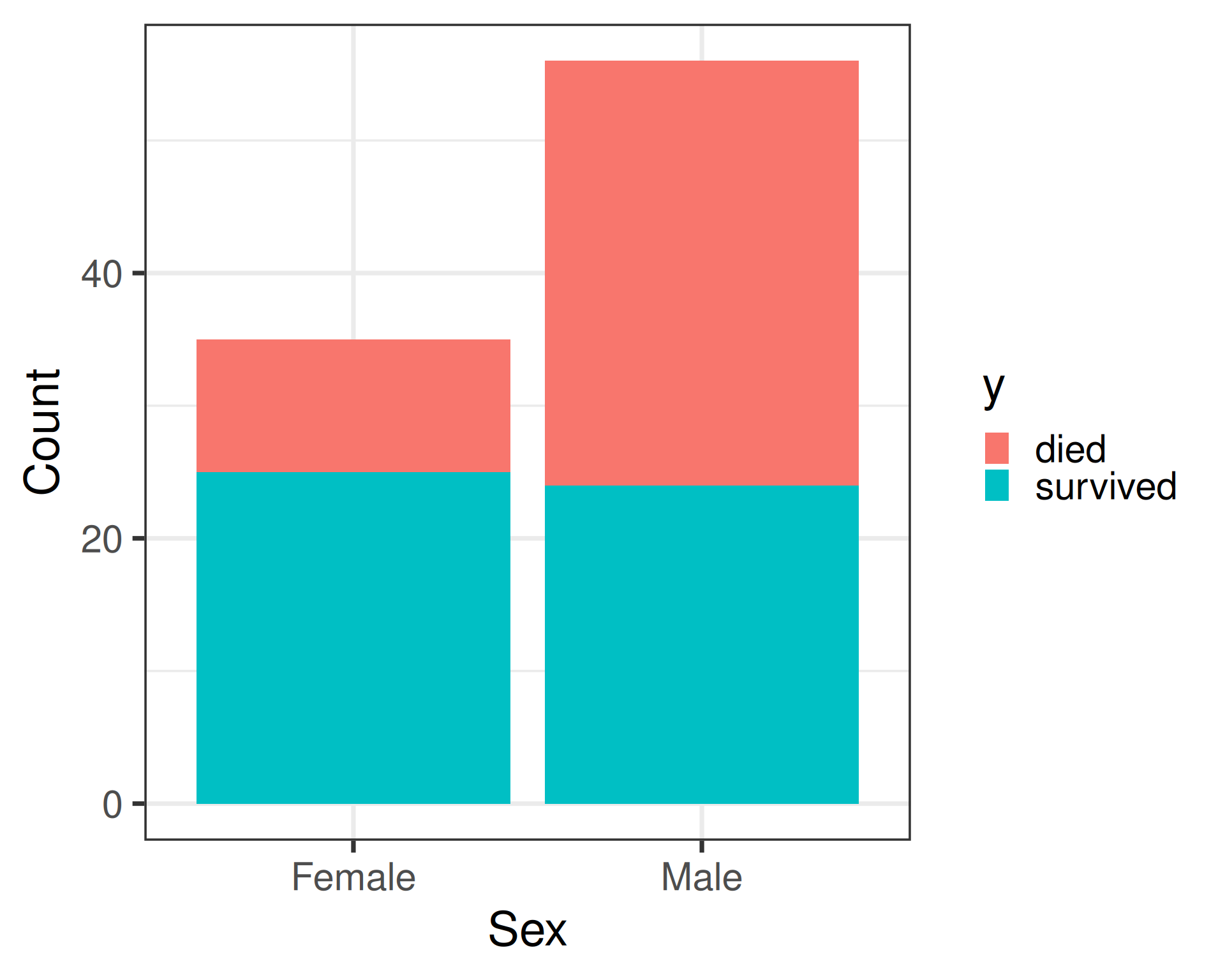
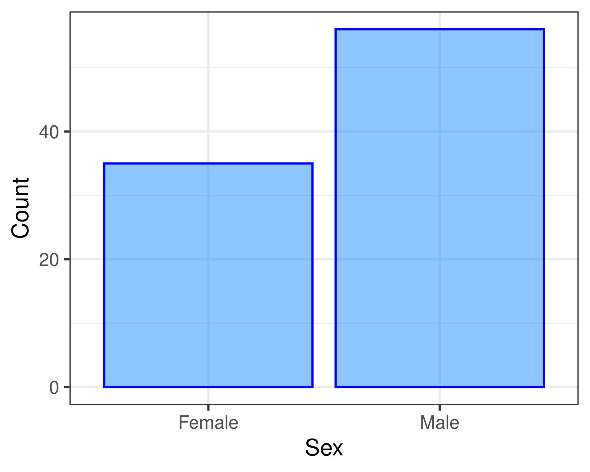
• Of the 91 individuals who set out with the Donner Party:

  • 42 (46.2%) died
  • 49 (53.8%) survived

Research Question

What characteristics might be associated with or predict survival?

Example: summary statistics

• Explanatory variable (\(x\)): sex (“male” or “female”)
• Response variable (\(Y\)): survival status (“survived” or “died”)

Binary response variable

A binary response variable takes on one of two values:

• Ex: survived vs. died; heart attack vs. no heart attack; yes vs. no
• Response of interest often labeled a “success” \[ Y_i = \begin{cases} \ 1 & \text{if obs. }i \text{ is a success}\\ \ 0 & \text{if obs. }i \text{ is not a success (i.e., a failure)} \end{cases} \]

The Bernoulli Distribution

\(Y_i\) is the outcome of a weighted coin flip, where

\[\begin{alignat*}{2} \Pr(Y_i = 1) &= \pi \quad &&\leftarrow \text{proportion of "successes"}\\ \Pr(Y_i = 0) &= 1 - \pi \quad &&\leftarrow \text{proportion of "failures"} \end{alignat*}\]

Important properties:

• \(\pi\): probability of success
• Mean: \(\mathbb{E}[Y_i] = P(Y_i = 1) = \pi\)
• Variance: \(Var(Y_i) = \pi(1-\pi)\)

Sidebar: Bernoulli vs. Binomial

Your textbook moves back and forth between two related—but not interchangeable—ways of reporting on binary data:

1. Individual result of each coin flip \(\implies\) Bernoulli
2. Cumulative results of \(n\) coin flips \(\implies\) Binomial

Ungrouped Binary Data

donner |>
  select(sex, age, y) |>
  head(15)

                              sex age        y
Breen_Edward_                Male  13 survived
Breen_Margaret_Isabella    Female   1 survived
Breen_James_Frederick        Male   5 survived
Breen_John                   Male  14 survived
Breen_Margaret_Bulger      Female  40 survived
Breen_Patrick                Male  51 survived
Breen_Patrick_Jr.            Male   9 survived
Breen_Peter                  Male   3 survived
Breen_Simon_Preston          Male   8 survived
Donner_Elitha_Cumi         Female  13 survived
Donner_Eliza_Poor          Female   3 survived
Donner_Elizabeth_Blue_Hook Female  45     died
Donner_Frances_Eustis      Female   6 survived
Donner_George                Male  61     died
Donner_George_Jr.            Male   9 survived

Grouped Binary Data

donner |> 
  summarize(
    survived = sum(y == "survived"),
    died = sum(y == "died"),
    total = n()
  )

  survived died total
1       49   42    91

# Grouped representation, with groups based on sex
donner |>
  group_by(sex) |>
  summarize(
    survived = sum(y == "survived"),
    died = sum(y == "died"),
    total = n()
  )

# A tibble: 2 × 4
  sex    survived  died total
  <fct>     <int> <int> <int>
1 Female       25    10    35
2 Male         24    32    56

The Binomial distribution

\(Y_i\) is the sum of \(n\) weighted coin flips, where

• \(n\): number of flips
• \(p\): probability of success

Important properties:

• Mean: \(\mathbb{E}[Y_i] = np\)
• Variance: \(Var(Y_i) = np(1-p)\)

Measures of frequency

• Probability:
  • Always between 0 and 1!
  • Ex: the chance that a woman survives the winter is 80%
  • Ex: If there were 10 women on the expedition, we would expect 8 of them to survive
• Odds:
  • unbounded
  • Ex: the chance that a woman survives the winter is 4 times as large as the chance that she does not
  • Ex: For each woman who dies, we expect 4 to survive

There and back again

• odds of success (\(\theta\)) and the probability of success (\(\pi\)) encode the exact same information
• \(\iff\) if we have one, we can always calculate the other!

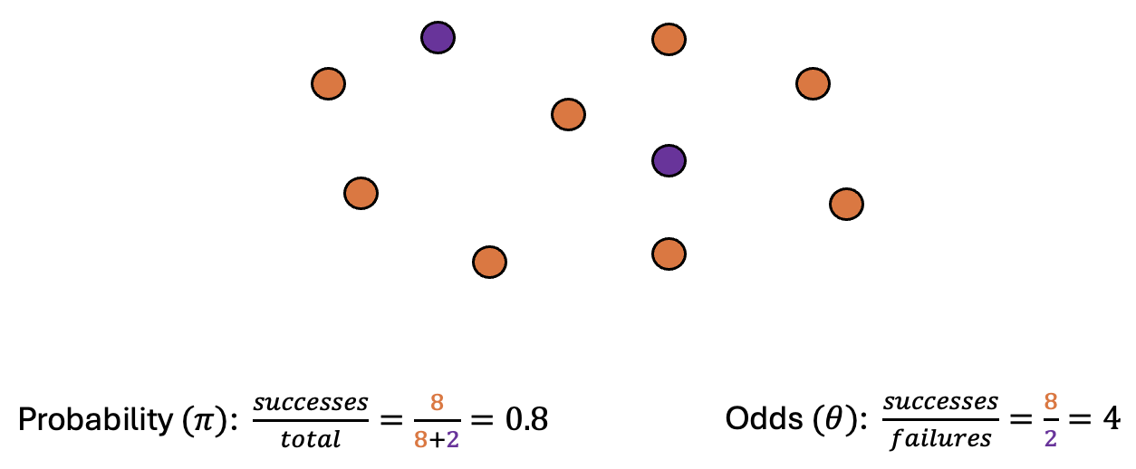
If we know the probability of success, \(\pi\)… \[ \theta = \frac{\pi}{ 1 - \pi} \]

If we know the odds of success, \(\theta\)… \[ \pi = \frac{\theta}{1 + \theta} \]

Measures of association: odds ratio

An odds ratio is a way to express the relationship between a binary response variable \(Y\) and an explanatory variable \(x\)

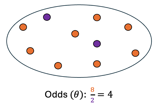
Women

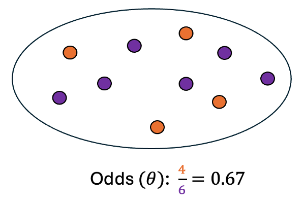
Men

• Odds ratio: a ratio of odds across two groups or populations \(\iff\) compares the frequency of “successes” between subpopulations

Contingency tables

• Show how counts of the binary response variable (\(Y\)) differ between two or more groups (\(x\)):

	Success (\(Y = 1\))	Failure (\(Y = 0\))
Group 1 (\(x = 1\))	a	b
Group 2 (\(x = 0\))	c	d

1. Estimating the probability of “success”:

\[\begin{align*} \widehat{\pi}(x = 1) &= \widehat{\Pr}(Y_i = 1 | x_i = 1) \\ &= \frac{a}{a + b} \\ &= \frac{\text{# successes in Group 1}}{\text{# observations in Group 1}} \end{align*}\]

2. Estimating the odds of “success”:

\[\begin{align*} \widehat{\theta}(x = 1) &= \frac{\widehat{\Pr}(Y_i = 1 | x_i = 1)}{\widehat{\Pr}(Y_i = 0 | x_i = 1)} \\ &= \frac{a/(a+b)}{b/(a +b)} \\ &= \frac{a}{b} \\ &= \frac{\text{# successes in Group 1}}{\text{# failures in Group 1}} \end{align*}\]

3. Estimating the odds ratio…

…for “success” in Group 1 compared to Group 2:

\[\begin{align*} \widehat{OR} &= \frac{\widehat{\theta}(x = 1)}{\widehat{\theta}(x = 0)} \\ &= \frac{\widehat{\pi}(x = 1)/ (1 - \widehat{\pi}(x = 1))}{\widehat{\pi}(x=0)/ (1 - \widehat{\pi}(x=0) )} \\ &= \frac{ad}{bc} \end{align*}\]

Interpretation of the Odds (\(\theta\))

Generic Interpretation

Among the subpopulation of observational units that belong to the group with \(x = x^*\), the chance (likelihood/probability) of a success is \(\widehat{\theta}\) times as large as the chance (likelihood/probability) of a failure.

• Donner Party: Odds of Survival Among Men

Among men traveling with the Donner Party expedition, the probability of surviving the winter was 0.75 times as large as the probability of dying.

Interpretation of the Odds Ratio (\(OR\))

The odds of a success are \(\widehat{OR}\) times as large among the group with \(x = 1\) than among the group with \(x = 0\).

• \(OR > 1\): \((OR - 1)100\%\) increase in odds
• \(OR < 1\): \((1 - OR)100\%\) decrease in odds

Donner Party: Odd Ratio

The odds of survival were 0.3 times as large among male members of the Donner party as among female members of the party.

The odds of survival were 70% smaller for men than for women.

\[ \text{Scratch Work: } (1 - 0.3) \times 100\% = 0.7\times 100\% = 70\% \]

Inference for population odds ratio

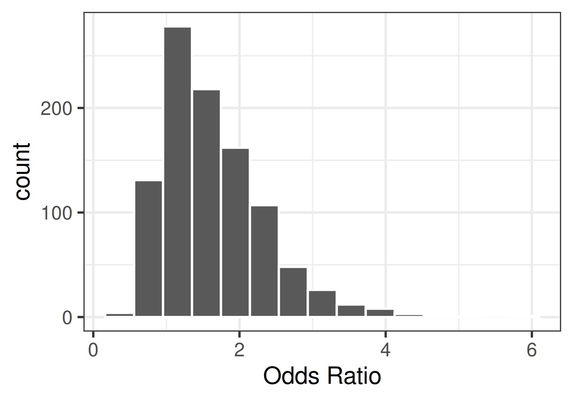
Formal statistical inference often works with the (natural) log of the odds ratio, since its sampling distribution is approximately Normal in sufficiently large samples¹

1. Rule of thumb: at least 5 successes and at least 5 failures in each group!

Introducing the log odds ratio

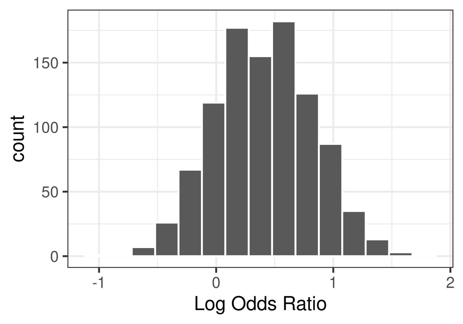
Working with the log odds ratio also allows us to convert division into subtraction (and vice versa): \[ \log(\widehat{OR}) = \log{\frac{\widehat{\theta}(1)}{\widehat{\theta}(0)}} = \log{ \widehat{\theta}(1) } - \log{ \widehat{\theta}(0) } \]

So we can find the log odds ratio by taking the difference of the log odds…

# Difference in the log odds
log(0.75) - log(2.5)

[1] -1.203973

# Log of the odds ratio
log(0.75 / 2.5)

[1] -1.203973

…And then exponentiate this difference to find the odds ratio!

# Exponentiating difference in log odds
exp(log(0.75) - log(2.5))

[1] 0.3

# Odds ratio
0.75 / 2.5

[1] 0.3

Inference for population odds ratio

Confidence Intervals for the Odds Ratio

Given the observed data, what is a range of plausible values for the true population odds ratio?

• Point Estimate: \(\log(\widehat{OR}) = \log(ad/bc)\)
• Standard Error: \(SE(\log(\widehat{OR})) = \sqrt{\frac{1}{a} + \frac{1}{b} + \frac{1}{c} + \frac{1}{d}}\)

• \(100(1-\alpha)\)% Confidence Interval for the Log Odds Ratio: \[ \log(\widehat{OR}) \pm z^* \cdot SE(\log(\widehat{OR})) \]

• \(100(1-\alpha)\)% Confidence Interval for the Odds Ratio:

\[ \left(e^{\log(\widehat{OR}) - z^* SE\{\log(\widehat{OR})\}}, \ e^{\log(\widehat{OR}) + z^* SE\{\log(\widehat{OR})\}}\right) \]

Summary

	Probability	Odds	Odds Ratio
Measures	Frequency	Frequency	Association
Compares:	Ratio of part to whole	Ratio of success to failure	Odds of success across two groups (Group 1/Group 2)
Range:	\((0, 1)\)	\((0, \infty)\)	\((0, \infty)\)
Successes More Common:	\(\pi > 0.5\)	\(\theta > 1\)	In Group 1 when \(OR > 1\)
Equal Likelihood:	\(\pi = 0.5\)	\(\theta = 1\)	\(OR = 1\)
Failures More Common:	\(\pi < 0.5\)	\(\theta < 1\)	In Group 1 when \(OR < 1\)