21-Logistic Regression

SDS 291

Prof. Baumer

November 17, 2025

Motivating logistic regression

Contingency table analysis allows us to summarize the relationship between a binary categorical response, \(Y_i\), and a categorical explanatory variable, \(x_i\)

• What if we had a continuous explanatory variable instead?
• What if we wanted to simultaneously consider multiple possible explanatory variables?

Our Goal

Extend linear regression techniques to binary response variables in order to:

• Summarize patterns observed in the data
• Classify or predict values of the response
• Quantify and evaluate the relationship between teh explanatory variable(s) and the frequency of a success

Donner Party redux

Research Question

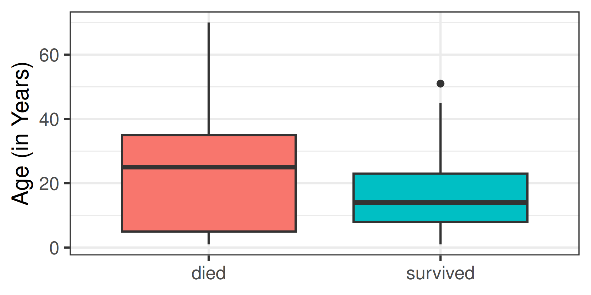
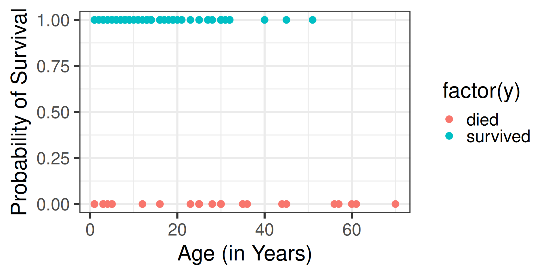
What characteristics might be associated with survival?

Note

Can we use linear regression techniques to model \(\mathbb{E}[Y_i | x_i] = \beta_0 + \beta_1 x_i\)? Why or why not?

Limitations of Linear Regression

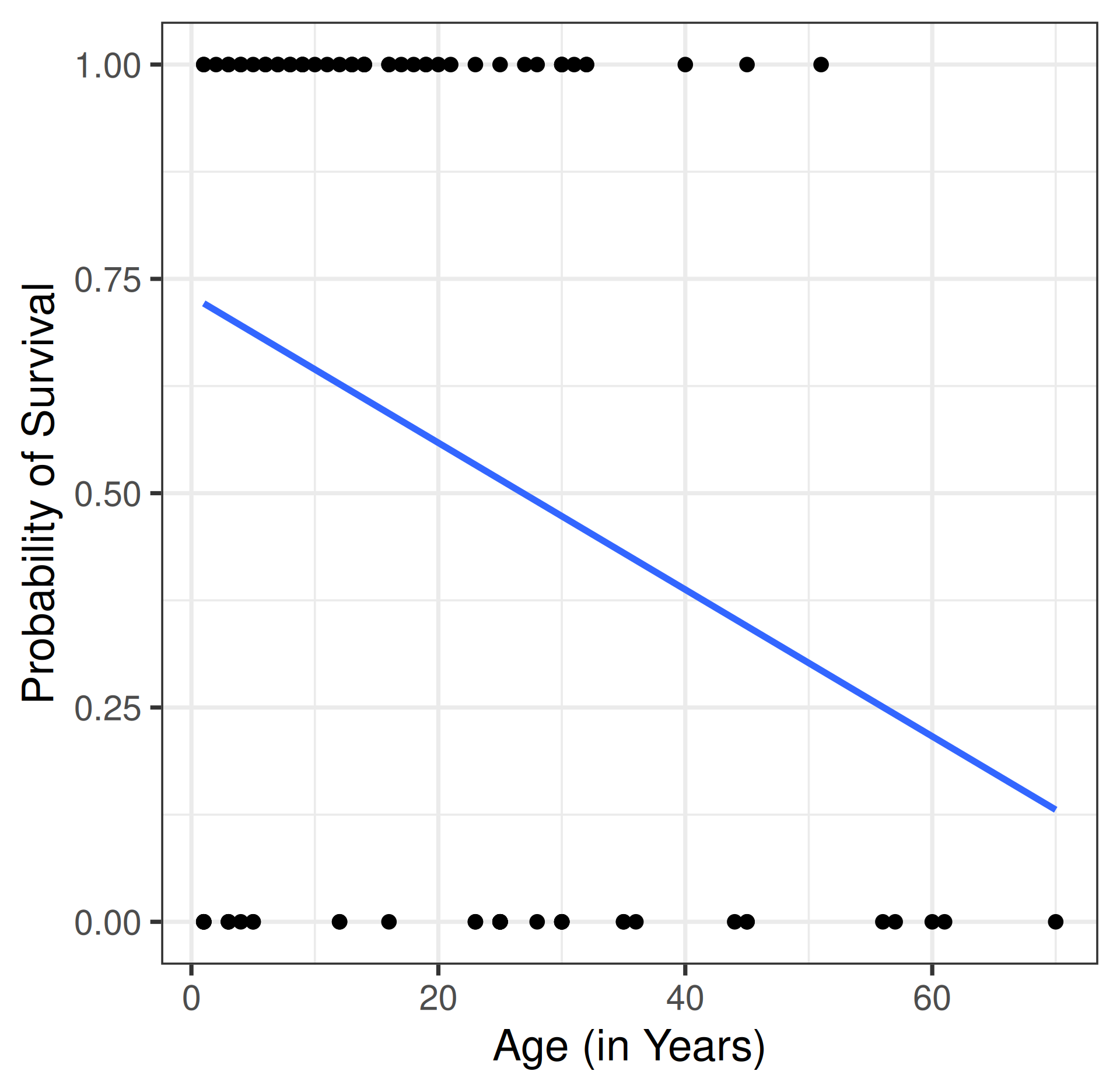
• Can produce predicted probabilities greater than 1 or less than 0!
• Response is not Normally distributed about the line
• Variance is no longer constant as a function of \(x\)

Generalized linear models (GLMs)

Link one or more explanatory variables to a function of the expected value of the response variable: \[g\left(\mathbb{E}[Y_i | x_i]\right) = \beta_0 + \beta_1 x_i\]

Three components of a GLM:

1. Random: What distribution does the response \(Y\) follow?
2. Predictor: What linear function of the explanatory variables?
3. Link function: What function \(g(\star)\) connects the linear predictor to the expected value of the response?

Link functions

• If link is the identity, \(g(\star) = \star\), then we model the mean as a linear combination of the explanatory variables: \[ g\left(\mathbb{E}[Y_i | x_i]\right) = \mathbb{E}[Y_i | x_i] = \beta_0 + \beta_1x_i \]

• If link is the logit, \(g(\star) = \text{logit}(\star) = \log(\frac{\star}{1-\star})\), then we model the log odds as a linear combination instead: \[\begin{align*} g\left( \mathbb{E}[Y_i | x_i]\right) =\text{logit}\left(E[Y_i | x_i]\right) &=\text{logit}\{\pi(x_i)\} \\ &= \log\left\{\frac{\pi(x_i)}{1 - \pi(x_i)}\right\} \\ &= \log\left\{\theta(x_i)\right\} = \beta_0 + \beta_1 x_i \end{align*}\]

The logistic regression model

Each person’s outcome is a weighted coin flip, where the probability that the coin lands heads, \(\pi(x)\), depends on one or more explanatory variables: \[ \text{logit}\left( \pi(x) \right) = \log{ \left( \frac{\pi(x)}{1 - \pi(x)} \right) } = \beta_0 + \beta_1x_1 +\beta_2x_2 + \cdots + \beta_kx_k \]

• Heads: the person experiences a “success”, \(Y_i = 1\)
• Tails: the person experiences a “failure”, \(Y_i = 0\)

Assumptions for Logistic Regression

1. The response variable \(Y_i\) is a Bernoulli random variable (i.e., a coin flip model makes sense)
2. All observations are independent of one another
3. There is a linear relationship between \(x\) and the log odds of a success

Re-expressing the logistic model

Linear function for the log-odds… \[ \log\left\{\theta(x_i)\right\} = \beta_0 + \beta_1 x_i \iff \theta(x_i) = e^{\beta_0 + \beta_1x_i} \]

…becomes a non-linear function for the success probability, \(\pi(x)\):

\[ \pi(x_i) = \frac{\theta(x_i)}{1 + \theta(x_i)} = \frac{e^{\beta_0 + \beta_1x_i}}{1 + e^{\beta_0 + \beta_1x_i}} \]

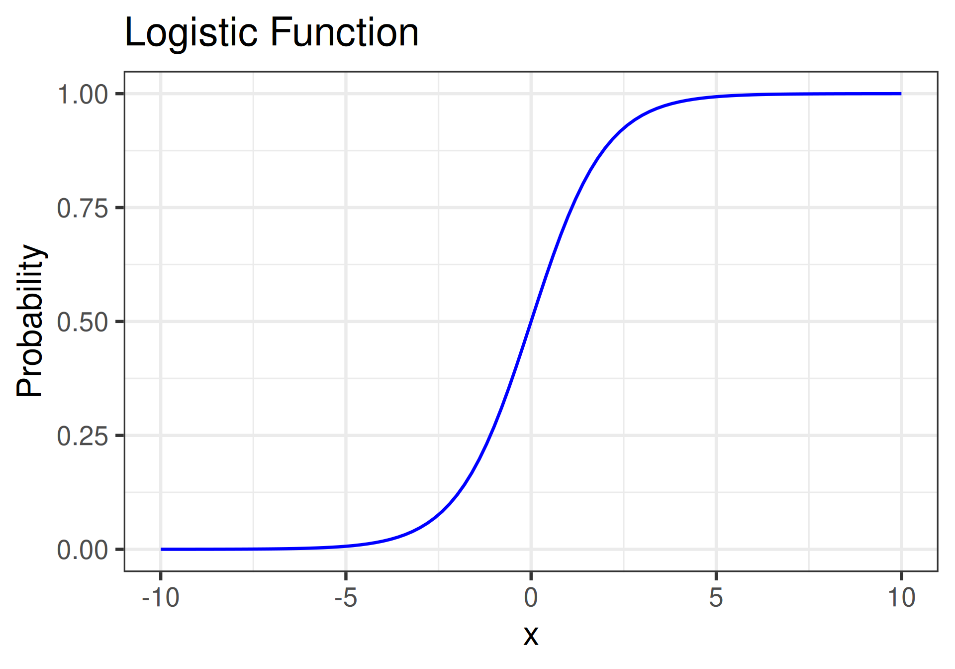
Three scales to consider

• on the probability scale:
  • units are easy to interpret
  • function is non-linear, which makes it hard to understand
• on the odds scale:
  • units are harder (but not impossible) to interpret
  • function is exponential, which makes it harder (but not impossible) to interpret
• on the log-odds scale:
  • units are nearly impossible to interpret
  • function is linear, which makes it easy to understand

Changing scales

log-odds scale:

\[\log{ \left( \frac{\pi(x_i)}{1 - \pi(x_i)} \right)} = \beta_0 + \beta_1x_i\]

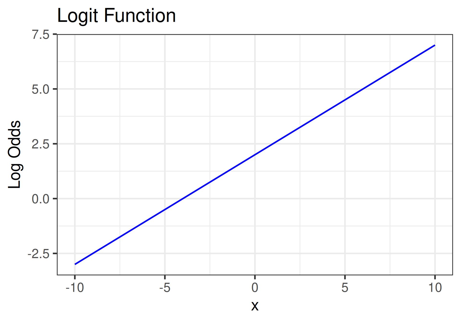
probability scale:

\[\pi(x_i) = \frac{e^{\beta_0 + \beta_1x_i}}{1 + e^{\beta_0 + \beta_1x_i}}\]

Comparisons with SLR

• How is a logistic regression model different than just log-transforming the response variable in a linear regression model?
• Throughout our discussion of linear regression, we frequently referenced the idea that \[ \text{data} = \text{model} + \text{random error} \]
• Where did the error term go in our logistic regression model?

Fitting a logistic regression model in R

Use the glm() function with family = "binomial"

donner_glm <- glm(y ~ age, data = donner, family = "binomial")
summary(donner_glm)

Call:
glm(formula = y ~ age, family = "binomial", data = donner)

Coefficients:
            Estimate Std. Error z value Pr(>|z|)   
(Intercept)  0.97917    0.37460   2.614  0.00895 **
age         -0.03689    0.01493  -2.471  0.01346 * 
---
Signif. codes:  0 '***' 0.001 '**' 0.01 '*' 0.05 '.' 0.1 ' ' 1

(Dispersion parameter for binomial family taken to be 1)

    Null deviance: 120.86  on 87  degrees of freedom
Residual deviance: 114.02  on 86  degrees of freedom
  (3 observations deleted due to missingness)
AIC: 118.02

Number of Fisher Scoring iterations: 4

Fitted Logit (Log-Odds) Form

\[ \text{logit}\{\widehat{\pi}(\texttt{age})\} = 0.979 - 0.037\left(\texttt{age}\right) \]

• Makes predictions about the log odds of survival
• Ex: The log-odds of survival are estimated to be 0.239 for 20-year-olds.

FItted Odds Form

\[ \widehat{\theta}(\texttt{age}) = e^{0.979 - 0.037\left(\texttt{age}\right)} \]

• Makes predictions about the odds of survival
• Ex: The odds of survival are estimated to be 1.270 for 20-year-olds.

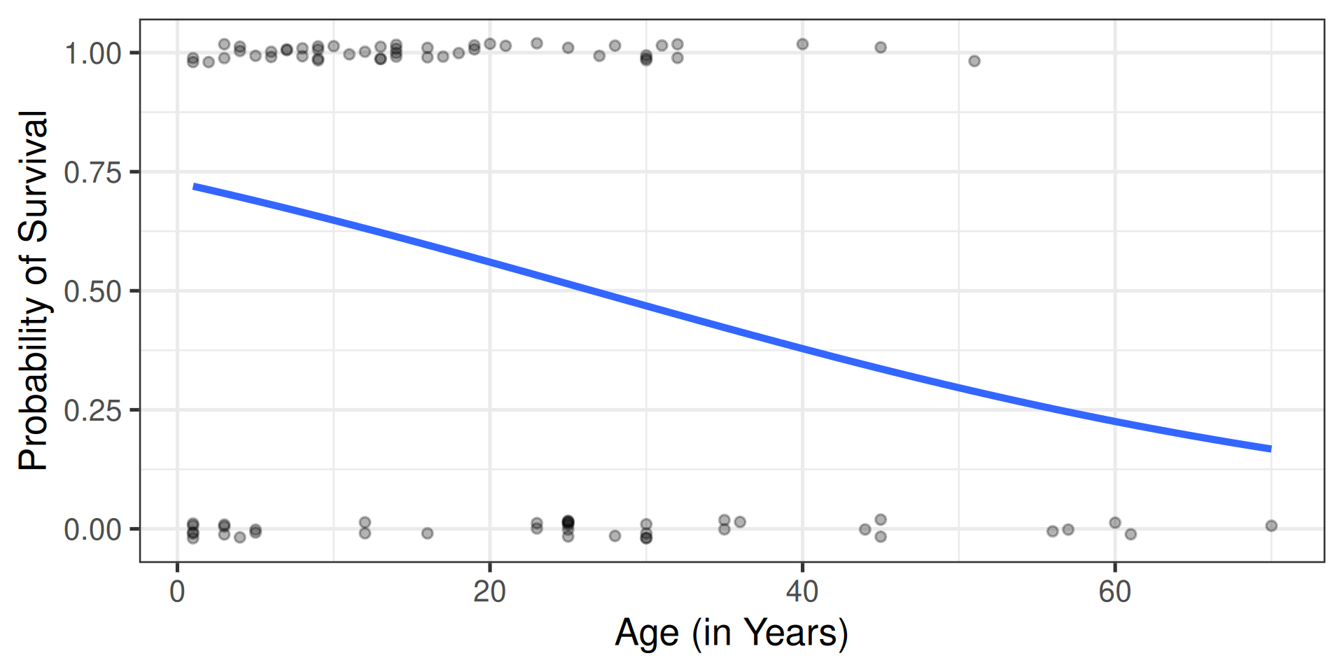
Fitted Logistic (Probability) Form

\[ \widehat{\pi}(\texttt{age}) = \frac{e^{0.979 - 0.037\left(\texttt{age}\right)}}{1 + e^{0.979 - 0.037\left(\texttt{age}\right)}} \]

• Makes predictions about the probability of survival
• Ex: The probability of survival is estimated to be 0.559 for 20-year-olds.

Coefficient interpretation: intercept

Tip

On the log odds scale, logistic regression looks like a linear model!

• Both the intercept and slope function like in linear regression
• Just need to transform them to the odds scale to make them interpretable!

• The intercept (when interpretable) still makes predictions about the subpopulation with \(x = 0\)
  • Summarizes the response variable using the (log) odds of success \[ \text{logit} ( \pi(0) ) = \beta_0 + \beta_1 (0) = \beta_0 \]

Coefficient interpretation: intercept

• Among the subpopulation of observational units for whom \(x_i = 0\), the odds of success are estimated to be \(e^{\widehat{\beta}_0}\).

Donner Party Intercept

• Among the Donner party members who were zero years old, the odds of survival are estimated to be 2.66. \[\text{Scratch Work: } e^{0.979} \approx 2.66\]

Coefficient interpretation: slope

• slope still captures associations between the explanatory and response variables
• Characterizes associations using the (log) odds ratio associated with a one-unit increase
• On the log-odds scale: \[\begin{align*} \text{logit}\left\{\pi(x^* + 1)\right\} &= \beta_0 + \beta_1(x^* + 1) \\ &= \text{logit}\left\{\pi(x^*)\right\} + \beta_1 \\ \log\{\theta(x^* + 1)\} - \log\{\theta(x^*)\} &= \beta_1 \\ \log\left(\theta(x^* + 1)/\theta(x^*)\right) &= \beta_1 \\ \log(OR) &= \beta_1 \end{align*}\]

Coefficient interpretation: intercept

• A one unit increase in the explanatory variable is associated with an estimated multiplicative change of \(e^{\widehat{\beta}_1}\) in the odds of success.

Donner Party Slope

• Among members of the Donner party, a one year increase in age was associated with an estimated 0.964 times change (3.6% decrease) in the odds of surviving the winter. \[\text{Scratch Work: } e^{-0.0369} \approx 0.964 \,\implies \, (1 - 0.964)\times 100\% = 3.6\%\]

Common interpretation pitfalls

1. Making interpretation additive rather than multiplicative

A one-year increase in age is associated with a 0.964 decrease in the odds of survival.

2. Making interpretation about probabilities rather than odds

A one-year increase in age is associated with a 0.964 times change in the probability [likelihood/chance/risk] of survival.

Making predictions in R

• type.predict = "link": returns predicted log-odds
• type.predict = "response": returns predicted probabilities

# Creating a data frame with the new values x* for age
new_ages <- data.frame(age = c(20, 40, 60))

# Predicted log odds (default)
donner_glm |>
  augment(
    newdata = new_ages,
#    type.predict = "link"
  )

# A tibble: 3 × 2
    age .fitted
  <dbl>   <dbl>
1    20   0.241
2    40  -0.496
3    60  -1.23 

# Predicted probabilities
donner_glm |>
  augment(
    newdata = new_ages,
    type.predict = "response"
  )

# A tibble: 3 × 2
    age .fitted
  <dbl>   <dbl>
1    20   0.560
2    40   0.378
3    60   0.225

Visualizing the fitted model

donner |> 
  ggplot(aes(x = age, y = ifelse(y == "survived", 1, 0))) +
  geom_jitter(alpha = 0.3, height = 0.02, width = 0, size = 2) +
  theme_bw(20) +
  xlab("Age (in Years)") +
  ylab("Probability of Survival") +
  geom_smooth(method = "glm", method.args = list(family = "binomial"), se = FALSE)

Comparison

Criterion	Linear Regression	Logistic Regression
Response Variable:	Continuous	Binary
Explanatory Variable(s):	Any type	Any type
Probability Model for Response Given \(x\):	Normal	Bernoulli/Binomial
\(\beta_0 + \beta_1 x\) Models:	Mean value of \(Y\)	Log odds of success
Coefficients:	Correspond to an additive change in the mean of \(Y\)	Need to be exponentiated in order to be meaningful. Correspond to a multiplicative change in the odds of success (\(Y = 1\))
Multiple Regression:	Interpretation now holding other explanatory variables constant	Interpretation now holding other explanatory variables constant