                          age        y    sex        family.name status
Murphy_Levinah_W._Jackson  36     died Female Murphy-Foster-Pike Family
Fosdick_Jay                23     died   Male             Graves Family
Donner_Samuel               4     died   Male           J_Donner Family
Donner_Elitha_Cumi 13 survived Female G_Donner Family22-Inference for Logistic Regression
SDS 291
Prof. Baumer
November 19, 2025
Model estimation (linear regression)
Once Upon a Time…
Because linear regression models have the framework \[ data = model + \text{random error}, \] we fit linear regression models by finding values for \(\widehat{\beta}_0\) and \(\widehat{\beta}_1\) that minimized this error: \[ \min_{\widehat{\beta}_0, \widehat{\beta}_1}{SSE} = \min_{\widehat{\beta}_0, \widehat{\beta}_1}{\sum_{i=1}^{n}e_i^2} = \min_{\widehat{\beta}_0, \widehat{\beta}_1}{\sum_{i=1}^{n}(y_i - \widehat{\beta}_0 - \widehat{\beta}_1x_i)^2} \] The resulting sum of squares decomposition informed how we assessed model fit and conducted inference!
Model estimation (logistic regression)
- Our logistic regression model doesn’t have explicit additive errors anymore
- \(\implies\) randomness instead comes from the coin flip model for the data
- We will need to take a different approach to fit our model!
The magician’s dilemma
Suppose you flip a weighted coin four times and see \[ Tails, \ Tails, \ Tails, \ Heads \]
If we knew the probability \(\pi\) that the coin landed on heads, then the probability of observing this sequence of outcomes would be
\[\begin{align*} \Pr(TTTH) &= \Pr(Y_1 = 0, Y_2 = 0, Y_3 = 0, Y_4 = 1) \\ &= \Pr(Y_1 = 0) \cdot \Pr(Y_2 = 0) \cdot \Pr(Y_3 = 0) \cdot \Pr(Y_4 = 0) \\ &= (1-\pi)(1-\pi)(1-\pi)\pi \\ &= (1 - \pi)^3 \pi \end{align*}\]
Note
But if we don’t actually know the value of \(\pi\), how can we find an estimate for it that makes the most sense with the observed data?
The likelihood
Given a particular probability model for how the data were generated (like our coin flip model for Bernoulli response variables),
- Likelihood: the probability of the observed data, regarded as a function of the unknown parameter(s) \[ \mathcal{L}(\pi) = \Pr(Y_1 = 0, Y_2 = 0, Y_3 = 0, Y_4 = 1) = (1-\pi)^3\pi \]
- Log-likelihood: the natural log of the likelihood function, which is often computationally easier to work with (sums \(>\) products) \[ \ell(\pi) = \log\mathcal{L}(\pi) = 3\log(1-\pi) + \log(\pi) \]
Coin flip likelihood function
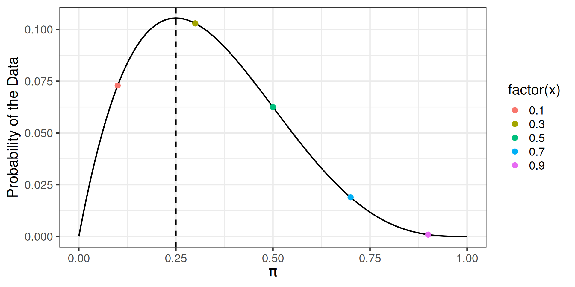
Maximum Likelihood Estimation
- Maximum likelihood estimator (MLE): the value of \(\pi\) that maximizes the log-likelihood
- makes the observed data most probable
- still trying to minimize the discrepancy between our estimated model and the observed data!
- just doing it in a different way!
How do we find the MLE?
- Use calculus!
- Take derivative of \(\ell\) (with respect to \(\pi\))
- Set equal to 0 and solve for \(\pi\)
\[ \frac{d \ell}{d \pi} = -\frac{3}{1-\pi} + \frac{1}{\pi} = 0 \implies \pi = \frac{1}{4} \]
The value of \(\pi\) that makes the observed data the most likely is \[ \widehat{\pi}_{MLE} = \frac{1}{4} \]
Likelihood for logistic regression
- \(\pi\) is no longer fixed, but depends on \(\beta_i\)’s
- Need to find MLE for \(\beta_i\)’s
\[ \mathcal{L}_i(\beta_0, \beta_1) = \pi(x_i) = \frac{e^{\beta_0 + \beta_1x_i}}{1 + e^{\beta_0 + \beta_1x_i}} \]
- For all \(n\) observations:
\[ \mathcal{L}(\beta_0, \beta_1) = \prod_{i=1}^{n}\left(\frac{e^{\beta_0 + \beta_1 x_i}}{1 + e^{\beta_0 + \beta_1 x_i}}\right)^{y_i}\left(\frac{1}{1 + e^{\beta_0 + \beta_1 x_i}}\right)^{1-y_i} \]
Likelihood for Donner Party sample
Suppose we looked at just four rows of the Donner Party data:
\[\begin{align*} \mathcal{L}(\beta_0, \beta_1) &= \Pr(Y_1 = 0, Y_2 = 0, Y_3 = 0, Y_4 = 1)\\ &= (1 - \pi(x_1)) (1 - \pi(x_2)) (1-\pi(x_3)) \pi(x_4) \\ &= (1 - \pi(36)) (1 - \pi(23)) (1-\pi(4) ) \pi(13) \\ &= \left( \frac{1}{1 + e^{\beta_0 + \beta_1(36)}} \right) \left(\frac{1}{1 + e^{\beta_0 + \beta_1(23)}} \right) \left(\frac{1}{1 + e^{\beta_0 + \beta_1(4)}} \right) \left(\frac{e^{\beta_0 + \beta_1(13)}}{1 + e^{\beta_0 + \beta_1(13)}} \right) \end{align*}\]
The likelihood for a logistic model
[1] 1.0000000 1.0000000 0.9933071 0.9999992Comparing to the fitted model in R
\[\text{logit}\left\{\widehat{\pi}(\texttt{age}_i)\right\} = 0.979 - 0.037\left(\texttt{age}_i\right)\]
Call:
glm(formula = y ~ age, family = "binomial", data = donner)

Coefficients:
            Estimate Std. Error z value Pr(>|z|)
(Intercept)  0.97917    0.37460   2.614  0.00895 **
age         -0.03689    0.01493  -2.471  0.01346 *
---
Signif. codes:  0 '***' 0.001 '**' 0.01 '*' 0.05 '.' 0.1 ' ' 1

(Dispersion parameter for binomial family taken to be 1)

    Null deviance: 120.86  on 87  degrees of freedom
Residual deviance: 114.02  on 86  degrees of freedom
  (3 observations deleted due to missingness)
AIC: 118.02

Number of Fisher Scoring iterations: 4
What’s so great about MLEs?
When we have a sufficiently large sample size…
- They are essentially unbiased, meaning that they (on average) give us the correct (true) answer
- Standard errors can be easily computed
- They have relatively small variability from sample to sample compared to other estimators
- Their sampling distribution is approximately Normal
Note
This last observation—and the likelihood more generally—forms the basis for inference with logistic regression models!
Inference for logistic regression
- Confidence Intervals: what is a range of plausible values for the true odds ratio for the association between \(x\) and \(Y\)?
- Hypothesis Tests: is the explanatory variable related to the frequency of successes in the population?
- Wald test: can be used to test a single coefficient or a weighted combination of coefficients
- Asks: Is the true population odds ratio relating \(x\) to \(Y\) equal to 1?
- Linear regression analog: \(t\)-tests
- Likelihood ratio test: can be used to compare any two nested models
- Asks: Is the simpler model for \(\pi(x)\) sufficient?
- Linear regression analog: nested \(F\)-tests
- Wald test: can be used to test a single coefficient or a weighted combination of coefficients
Wald tests for individual coefficients
Note
Is the true population odds ratio relating \(x\) to \(Y\) equal to 1?
- Formulate competing hypotheses: \[H_0: OR = 1 \text{ vs. } H_A: OR \neq 1 \iff H_0: \beta_1 = 0 \text{ vs. } H_A: \beta_1 \neq 0\]
- Determine a test statistic and its null distribution: \[z = \frac{\widehat{\beta}_1 - 0}{SE(\widehat{\beta}_1)} \ \overset{H_0}{\sim} \ N(0, 1)\]
Wald CIs for individual coefficients
Note
Because our regression coefficients encode log-odds ratios, we still follow our tried-and-true approach to build a CI for the \(\log(OR)\) first, \[\text{point estimate}\ \pm\ \text{margin of error} \quad \iff \quad \widehat{\beta}\ \pm\ z^*SE(\widehat{\beta})\] and then exponentiate to make our CI interpretable on the OR scale!
- 95% CI for the log odds ratio, \(\beta_1\): \[-0.037 \pm 1.96\left(0.015\right) = -0.037 \pm 0.0294 = (-0.066, -0.008)\]
- 95% CI for the odds ratio, \(e^{\beta_1}\):
\[(e^{-0.066}, e^{-0.008}) = (0.936, 0.992)\]
Caution: behavior of confint()
confint()doesn’t give the Wald interval
                2.5 %    97.5 %
(Intercept) 1.3072038 5.7380750
age 0.9341978 0.9910875- Workaround: use
confint.default()
Interpretation: We are 95% confident that a one year increase in age is associated with between 0.936 and 0.992 times the odds of surviving the Donner Party expedition (\(p = 0.013\))

SDS 291