23-Multiple Logistic Regression

SDS 291

Prof. Baumer

November 24, 2025

Recall: MLE

MLE: select the values for \(\widehat{\beta}_0\) and \(\widehat{\beta}_1\) that make the observed data the most likely
The maximized likelihood, \(\mathcal{L}_\text{model}\), gives us an alternative way of assessing model fit and testing (sets of) model coefficients!

Deviance: tool for assessing model fit

The deviance compares the likelihood of the observed data under the current fitted model to the likelihood of the data under a “saturated” model that matches the data exactly:

\[\begin{align*} \text{Deviance} &= -2\left\{\log\left(\mathcal{L}_\text{model}\right) - \log\left(\mathcal{L}_\text{saturated}\right)\right\}\\[0.3em] &= -2\log\left(\mathcal{L}_\text{model}\right) \ +\ \text{constant} \end{align*}\]

Will sometimes see the deviance written as just the first term
Intuition: how much does our model leave unexplained about the data relative to a perfect fit?
Linear regression analog: the error sum of squares, \(SSE\)

Tip

“Better” Models Have: smaller deviances

Deviance

Residual deviance (deviance for the current fitted model): functions like the error sum of squares (SSE)
“Null” deviance (deviance for the intercept-only model): functions like the total sum of squares (SST)


Call:
glm(formula = y ~ age, family = "binomial", data = donner)

Coefficients:
            Estimate Std. Error z value Pr(>|z|)   
(Intercept)  0.97917    0.37460   2.614  0.00895 **
age         -0.03689    0.01493  -2.471  0.01346 * 
---
Signif. codes:  0 '***' 0.001 '**' 0.01 '*' 0.05 '.' 0.1 ' ' 1

(Dispersion parameter for binomial family taken to be 1)

    Null deviance: 120.86  on 87  degrees of freedom
Residual deviance: 114.02  on 86  degrees of freedom
  (3 observations deleted due to missingness)
AIC: 118.02

Number of Fisher Scoring iterations: 4

Deviance \(\rightarrow\) AIC, BIC

Deviance forms the basis for how the AIC and BIC are defined for logistic regression and other GLMs

Akaike Information Criterion \[AIC = -2\left\{\log\left(\mathcal{L}_\text{model}\right)\right\} + 2\left(k + 1\right)\]
Schwarz’s Bayesian Information Criterion \[BIC = -2\left\{\log\left(\mathcal{L}_\text{model}\right)\right\} + \log(n)\left(k + 1\right)\]

# Finding metrics summarizing overall model fit
donner_glm |>
  glance()

# A tibble: 1 × 8
  null.deviance df.null logLik   AIC   BIC deviance df.residual  nobs
          <dbl>   <int>  <dbl> <dbl> <dbl>    <dbl>       <int> <int>
1          121.      87  -57.0  118.  123.     114.          86    88

Difference in deviances

Suppose that we want to compare two nested logistic regression models:

A more complicated, “full” model for \(\pi(x)\)
A less complicated, “reduced” model for \(\pi(x)\) that is formed by placing restrictions on the full model

How much information do we lose by using the simpler reduced model rather than the full model?

\[\begin{align*} G &=\text{Deviance}_\text{reduced} - \text{Deviance}_\text{full} \\ &= \Big\{-2\log\left(\mathcal{L}_\text{reduced}\right) \ +\ \text{constant}\Big\} - \Big\{-2\log\left(\mathcal{L}_\text{full}\right) \ +\ \text{constant}\Big\} \\ &= -2\left\{\log\left(\mathcal{L}_\text{reduced}\right) - \log\left(\mathcal{L}_\text{full}\right)\right\}\\ &= -2\log\left(\frac{\mathcal{L}_\text{reduced}}{\mathcal{L}_\text{full}}\right) \end{align*}\]

The (nested) likelihood ratio test

Note

Given two nested logistic regression models, how much less plausible is the observed data if we were to adopt the simpler model for \(\pi(x)\)?

The simpler model is an intercept-only model:

Formulate competing hypotheses:
- \(H_0: \text{logit}\left\{\pi(x)\right\} = \beta_0 \quad \text{vs.} \quad H_A: \text{logit}\left\{\pi(x)\right\} = \beta_0 + \beta_1 x\)
- \(H_0: \beta_1 = 0 \quad \text{vs.} \quad H_A: \beta_1 \neq 0\)
Determine a test statistic \[G =\text{Deviance}_\text{reduced} - \text{Deviance}_\text{full}\]

Visualizing the drop in deviance

\[H_0: \, \text{logit}\left\{\pi(x)\right\} = \beta_0\]

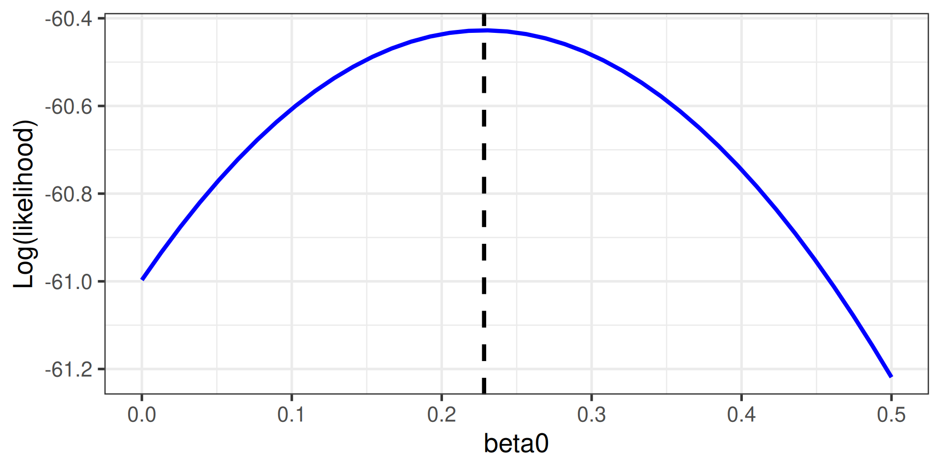
\[\begin{gather*} \log\left(\mathcal{L}_\text{reduced}\right) = -60.43\\ \text{Deviance}_\text{reduced} \approx 120.86 \end{gather*}\]

\[H_A: \, \text{logit}\left\{\pi(x)\right\} = \beta_0 + \beta_1x\]

\[\begin{gather*} \log\left(\mathcal{L}_\text{full}\right) = -57.01\\ \text{Deviance}_\text{full} \approx 114.02 \end{gather*}\]

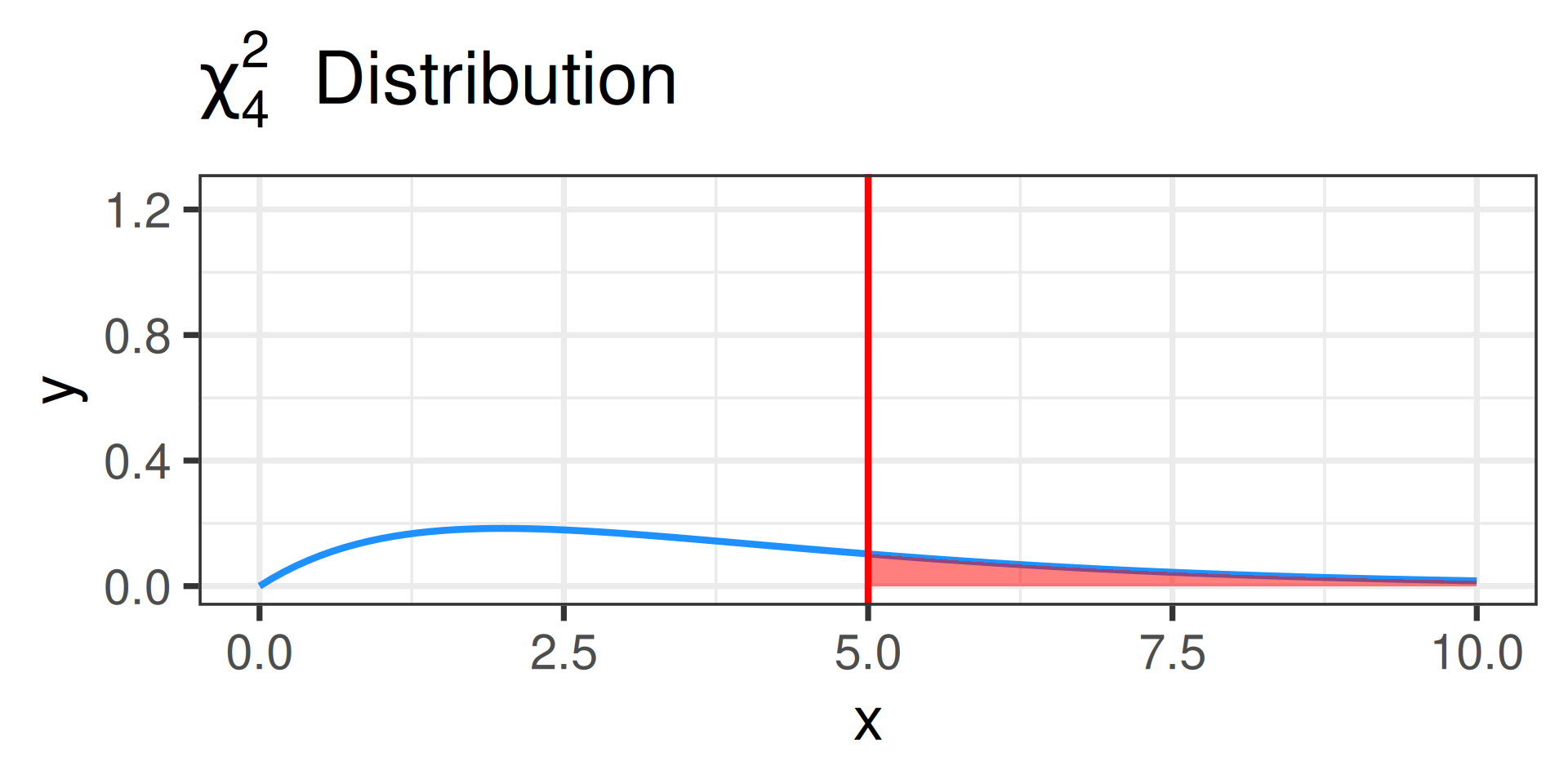
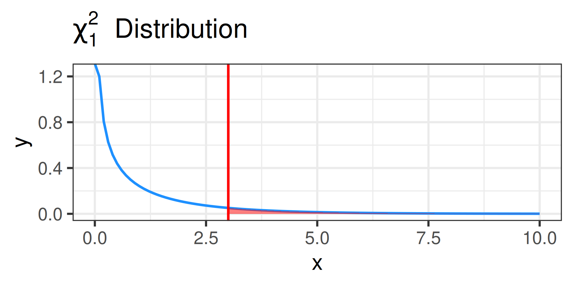
The \(\chi^2_p\) distribution

Under \(H_0\), the drop in deviance (\(G\)) follows a \(\chi^2_p\) distribution

Right-skewed distribution whose shape is controlled by one parameter: the degrees of freedom (\(p\))
\(p\) is the number of restrictions placed on the full model
\(p\)-value for the likelihood ratio test: \(\Pr(\chi^2_p \geq G)\)

Conducting the likelihood ratio test

donner_cc <- donner |> 
  filter(!is.na(age))
reduced_glm <- glm(y ~ 1, data = donner_cc, family = "binomial")

full_glm <- glm(y ~ age, data = donner_cc, family = "binomial")

# Calculating the test statistic
G <- reduced_glm$deviance - full_glm$deviance
G

[1] 6.836785

# Finding the p-value
pchisq(G, df = 1, lower.tail = FALSE)

[1] 0.008929939

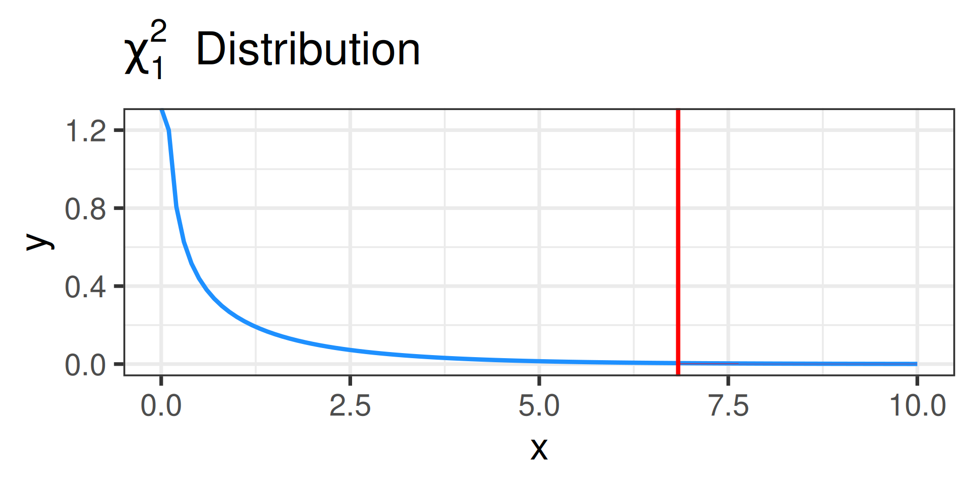
Visualizing the LRT

chi_plot +
  stat_function(fun = dchisq, args = list(df = 1), col = "dodgerblue", size = 1.5) +
  geom_vline(xintercept = G, col = "red", size = 1.5) +
  geom_area(stat = "function", fun = dchisq, args = list(df = 1), fill = "red", xlim = c(G, 10), alpha = 0.5)

In practice: LRT using `anova()`

Requires a test argument to indicate that we are using a chi-square distribution (\(\chi^2\)) as our null distribution
Produces an analysis of deviance table rather than an analysis of variance table

anova(reduced_glm, full_glm, test = "Chisq")

Analysis of Deviance Table

Model 1: y ~ 1
Model 2: y ~ age
  Resid. Df Resid. Dev Df Deviance Pr(>Chi)   
1        87     120.86                        
2        86     114.02  1   6.8368  0.00893 **
---
Signif. codes:  0 '***' 0.001 '**' 0.01 '*' 0.05 '.' 0.1 ' ' 1

Comparing Wald test and LRT

Both tests led us to the same overall conclusion:

We reject the null hypothesis and find a statistically significant relationship between age and survival on the Donner Party expedition at the \(\alpha = 0.05\) level

The two tests produced slightly different \(p\)-values, though!
- Wald test: \(p = 0.01346\), LRT: \(p = 0.00893\)
- Recall: exact equivalence between \(t\)- and \(F\)-tests for a single coefficient in linear regression
Tests will usually agree (especially if we have a large sample size)
- If there are discrepancies: LRT preferred

Reporting LRT \(p\)-values

By default, summary() reports Wald \(p\)-values only
To get LRT \(p\)-values for each variable, we can use the drop1() function with test = "Chisq"

drop1(full_glm, test = "Chisq")

Single term deletions

Model:
y ~ age
       Df Deviance    AIC    LRT Pr(>Chi)   
<none>      114.02 118.02                   
age     1   120.86 122.86 6.8368  0.00893 **
---
Signif. codes:  0 '***' 0.001 '**' 0.01 '*' 0.05 '.' 0.1 ' ' 1

Multiple logistic regression

\[ \text{logit}\{\pi(x_i)\} = \beta_0 + \beta_1x_{i1} + \beta_2x_{i2} + \cdots + \beta_k x_{ik} \]

Fitted coefficient values are conditional on the other variables in the model
Coefficients (\(\beta_{j}\)) capture the change in the log odds of success, holding all other explanatory variables constant
Exponentiated coefficients (\(e^{\beta_j}\)) capture the multiplicative change in the odds of success, holding all other explanatory variables constant

Note

Categorical predictors, interactions, and polynomial terms are all fair game!

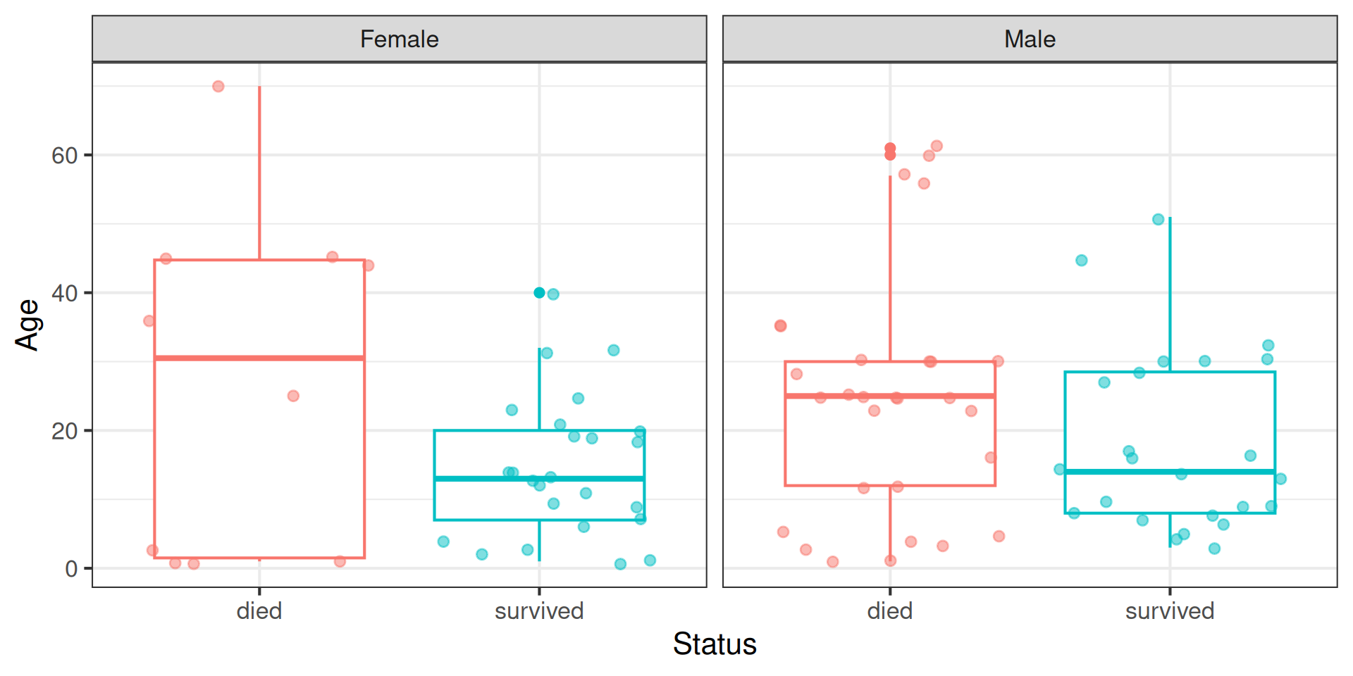
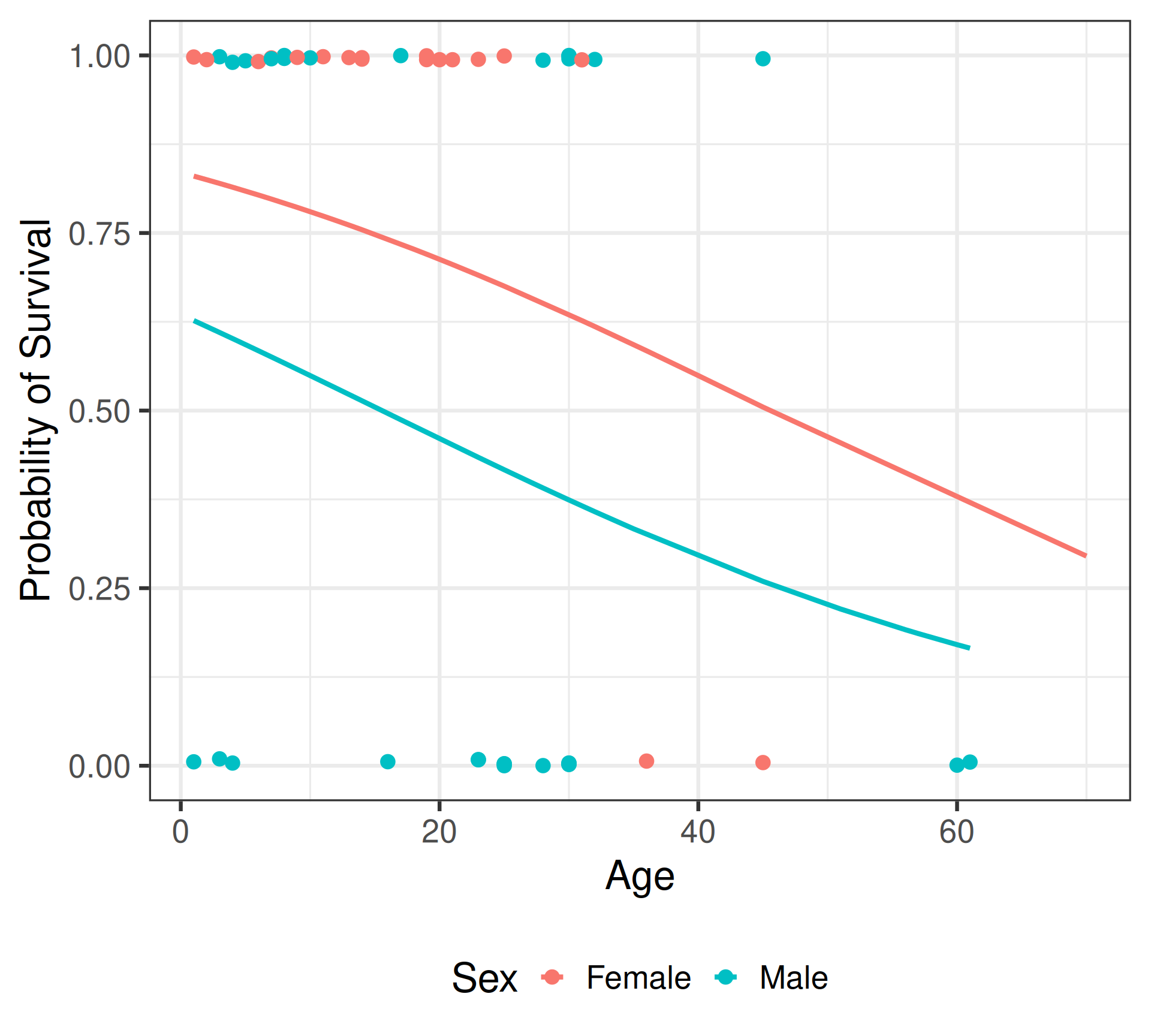
Ex: age and sex on the Donner party

Does the relationship between age and survival differ depending on sex?

Ex: additive model for Donner

Population Model

\[ \text{logit}\{\pi(\texttt{Age}_i, \texttt{Male}_i)\} = \beta_0 + \beta_1(\texttt{Age}_i) + \beta_2(\texttt{Male}_i) \]

Fitted Model

\[ \text{logit}\{\widehat{\pi}(\texttt{Age}_i, \texttt{Male}_i)\} = 1.622 - 0.036(\texttt{Age}_i) - 1.068(\texttt{Male}_i) \]

# Fitting the additive model
donner_age_sex <- glm(y ~ age + sex, data = donner, family = binomial)
summary(donner_age_sex)$coefficients

               Estimate Std. Error   z value    Pr(>|z|)
(Intercept)  1.62180162 0.50279192  3.225592 0.001257124
age         -0.03560529 0.01524512 -2.335521 0.019516239
sexMale     -1.06797669 0.48228705 -2.214401 0.026801239

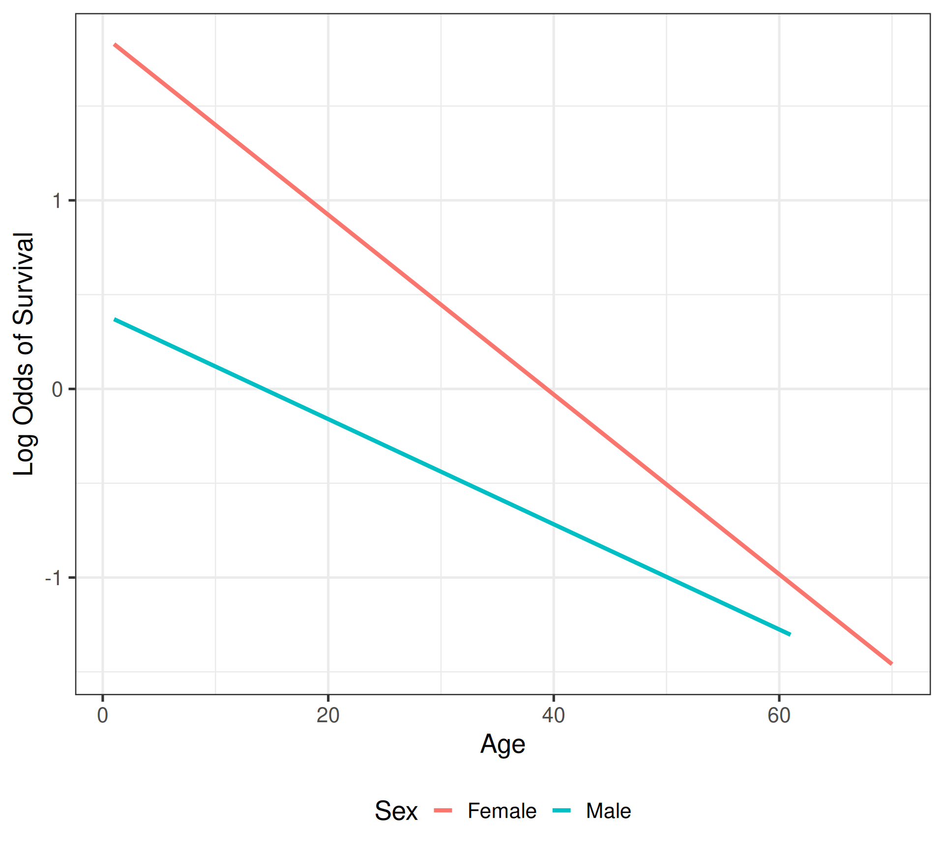
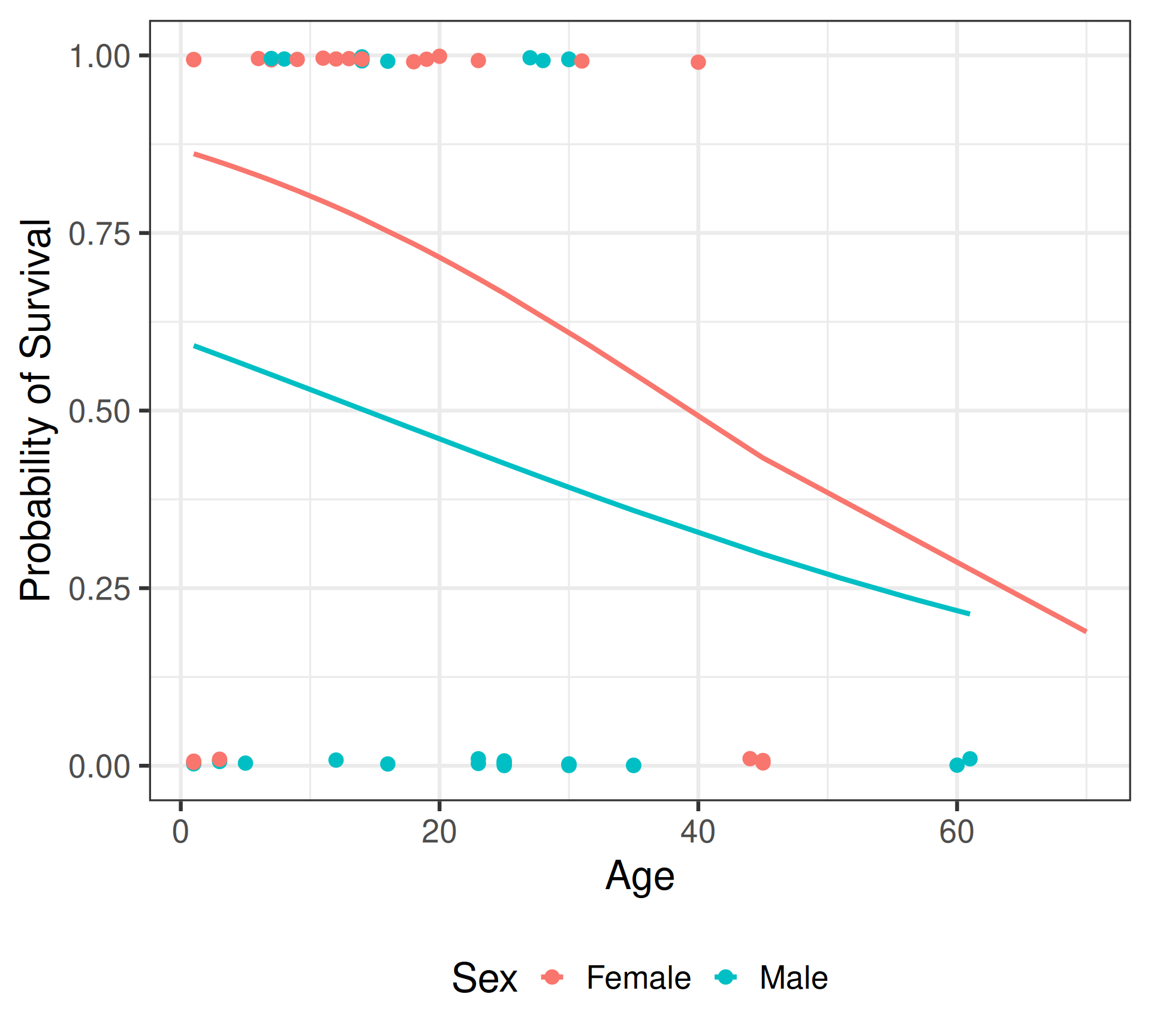
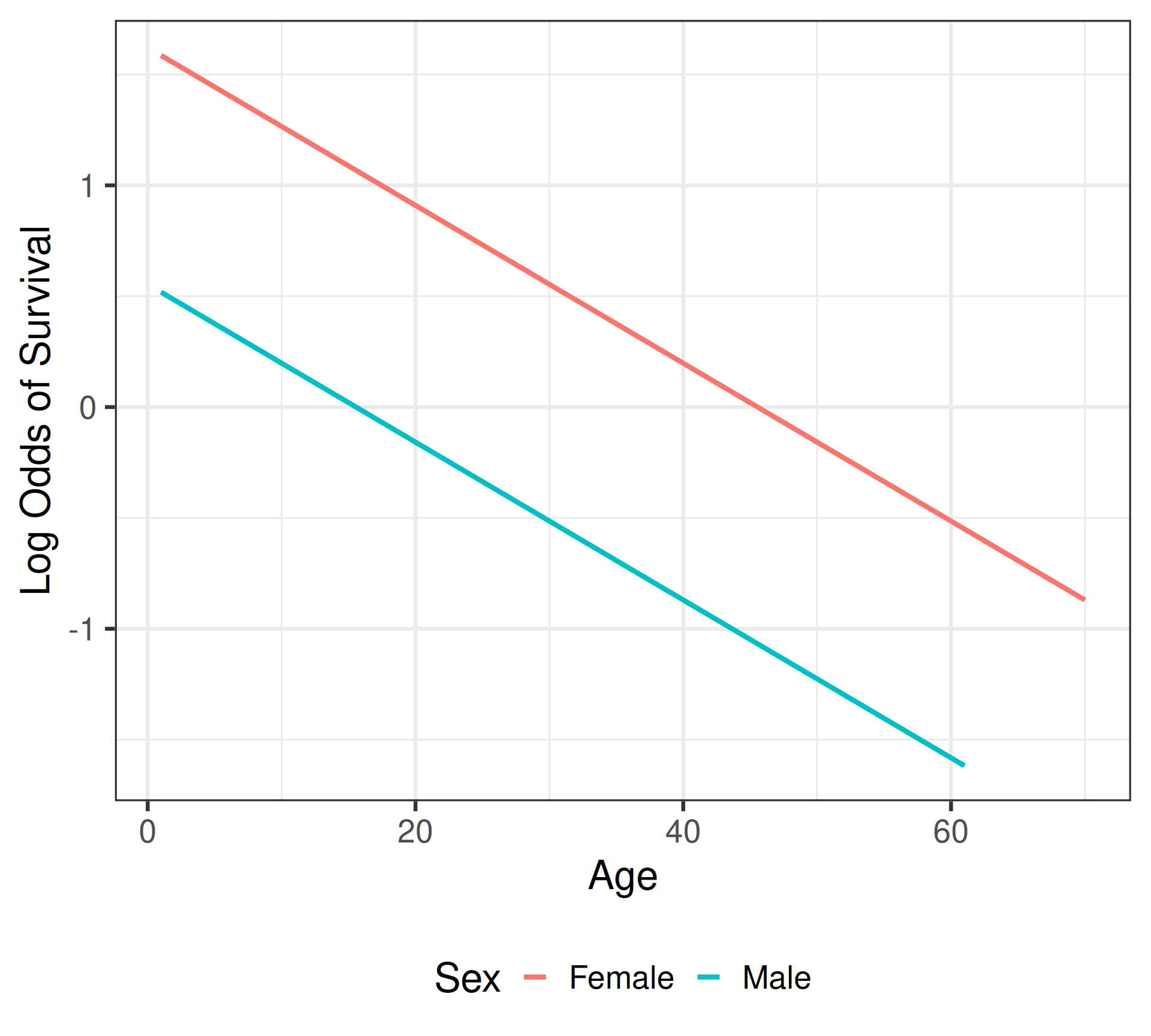
Visualizing the additive model

Fitted Model

\[ \text{logit}\{\widehat{\pi}(\texttt{Age}_i, \texttt{Male}_i)\} = 1.622 - 0.036(\texttt{Age}_i) - 1.068(\texttt{Male}_i) \]

Interpreting the additive model

Fitted Model

\[ \text{logit}\{\widehat{\pi}(\texttt{Age}_i, \texttt{Male}_i)\} = 1.622 - 0.036(\texttt{Age}_i) - 1.068(\texttt{Male}_i) \]

Intercept: the odds of survival for females who are 0 years old are estimated to be \(5.06\), i.e., for each 0-year-old female infant who dies, we expect 5.06 to survive \[\text{Scratch Work: }e^{1.622}\approx 5.06\]
Age: among individuals of the same sex, a one year increase in age is associated with an \(0.96\) times change in the odds of survival \[\text{Scratch Work: }e^{-0.036}\approx 0.96\]
Male: among individuals of the same age, the odds of survival are \(0.34\) times as high for males as for females \[\text{Scratch Work: }e^{-1.068}\approx 0.34\]

Incorporating an interaction

Interaction Model

Allow the association (slope) between age and the log odds of survival to differ based on sex:

\[ \text{logit}\{\pi(\texttt{Age}_i, \texttt{Male}_i)\} = \beta_0 + \beta_1(\texttt{Age}_i) + \beta_2(\texttt{Male}_i) + \beta_3(\texttt{Age}_i)(\texttt{Male}_i) \]

23-Multiple Logistic Regression

Recall: MLE

Deviance: tool for assessing model fit

Deviance

Deviance \(\rightarrow\) AIC, BIC

Difference in deviances

The (nested) likelihood ratio test

Visualizing the drop in deviance

The \(\chi^2_p\) distribution

Conducting the likelihood ratio test

Visualizing the LRT

In practice: LRT using anova()

Comparing Wald test and LRT

Reporting LRT \(p\)-values

Multiple logistic regression

Ex: age and sex on the Donner party

Ex: additive model for Donner

Visualizing the additive model

Interpreting the additive model

Incorporating an interaction

In practice: LRT using `anova()`