24-Classification Metrics

SDS 291

Prof. Baumer

December 1, 2025

Example: Malignant tunors

Identifying malignant tumors

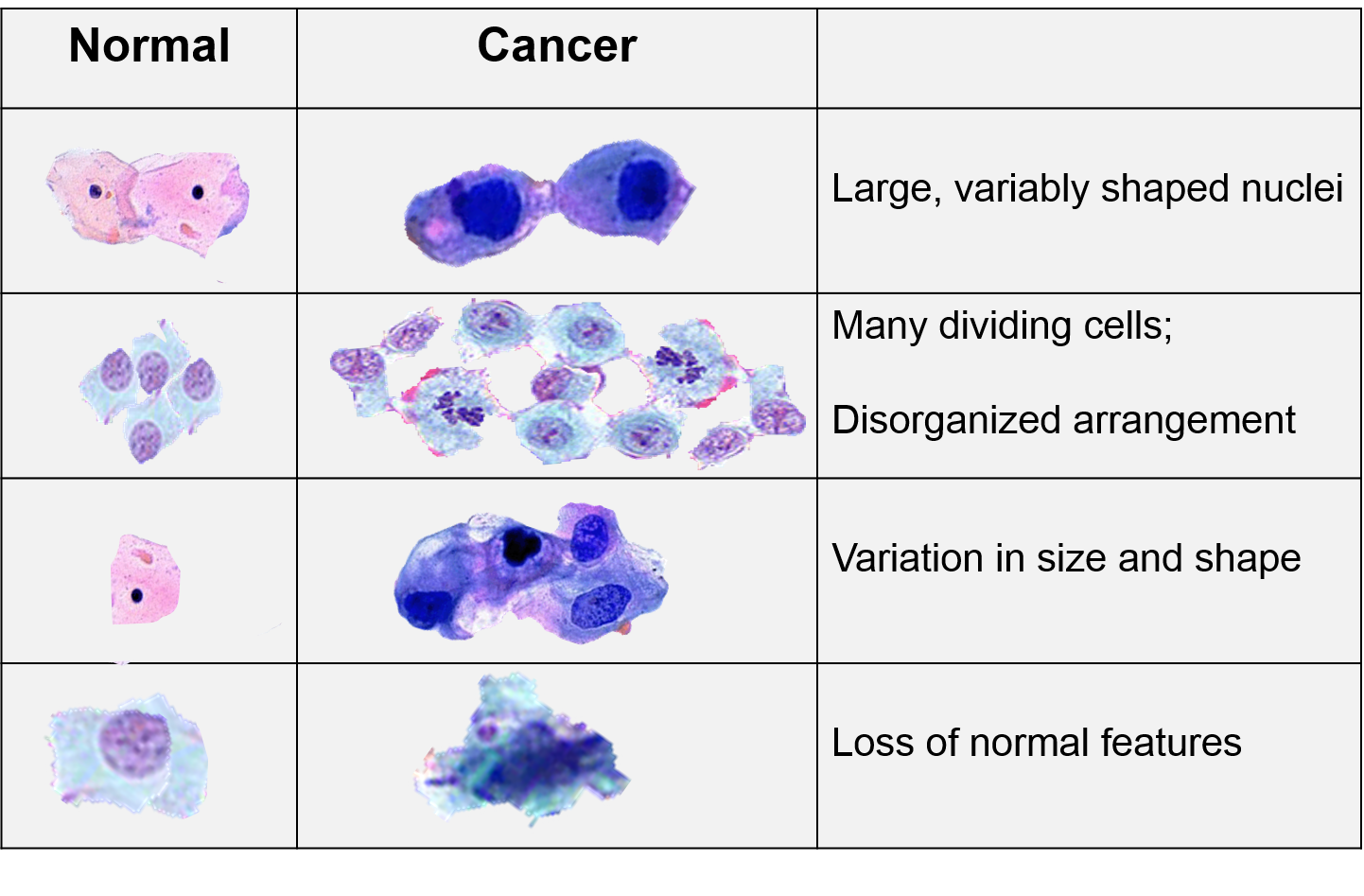
Suppose that oncologists…

…wish to build a model to predict which tumors are malignant (versus benign) based on the visual characteristics of the cells:

• Average radius of all visible cell nuclei (Radius)
• Indicator of whether the visible cell nuclei are misshapen and concave (Concave)

Logistic models

The linear predictor component of a GLM is the same in logistic and linear regression:

• Additive models incorporate information from both visual characteristics simultaneously
• Interaction models allow the relationship between the radius of the nuclei and tumor malignancy to differ depending on concavity (and for the nuclei shape/tumor malignancy relationship to differ depending on the radius!)

Additive model for tumor malignancy

Let \(\pi\) be the probability that a particular tumor is malignant

Population Model

\[ \text{logit}\left\{\pi(\texttt{Radius}, \texttt{Concave})\right\} = \beta_0 + \beta_1(\texttt{Radius}) + \beta_2(\texttt{Concave}) \]

Fitted Model

\[ \text{logit}\left\{\widehat{\pi}(\texttt{Radius}, \texttt{Concave})\right\} = -13.132 + 2.718(\texttt{Radius}) + 3.319(\texttt{Concave}) \]

Fitting the additive model

# Fitting the additive model
additive_glm <- glm(
  Malignant ~ Radius + Concave,
  data = cell,
  family = "binomial"
)
summary(additive_glm)

Call:
glm(formula = Malignant ~ Radius + Concave, family = "binomial", 
    data = cell)

Coefficients:
            Estimate Std. Error z value Pr(>|z|)    
(Intercept) -13.1320     1.4932  -8.795  < 2e-16 ***
Radius        2.7175     0.3663   7.418 1.19e-13 ***
Concave       3.3192     0.3545   9.362  < 2e-16 ***
---
Signif. codes:  0 '***' 0.001 '**' 0.01 '*' 0.05 '.' 0.1 ' ' 1

(Dispersion parameter for binomial family taken to be 1)

    Null deviance: 751.44  on 568  degrees of freedom
Residual deviance: 224.02  on 566  degrees of freedom
AIC: 230.02

Number of Fisher Scoring iterations: 7

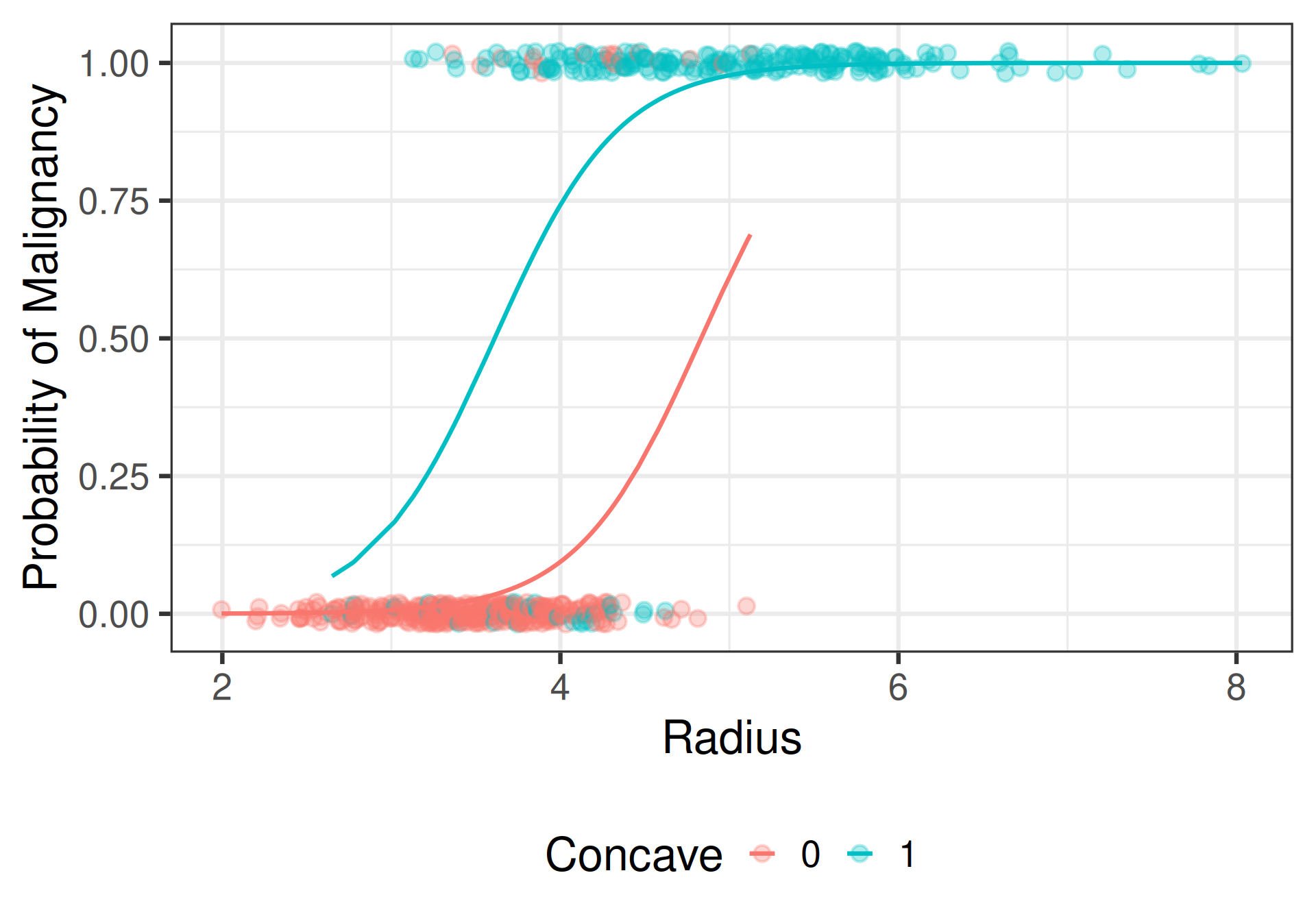
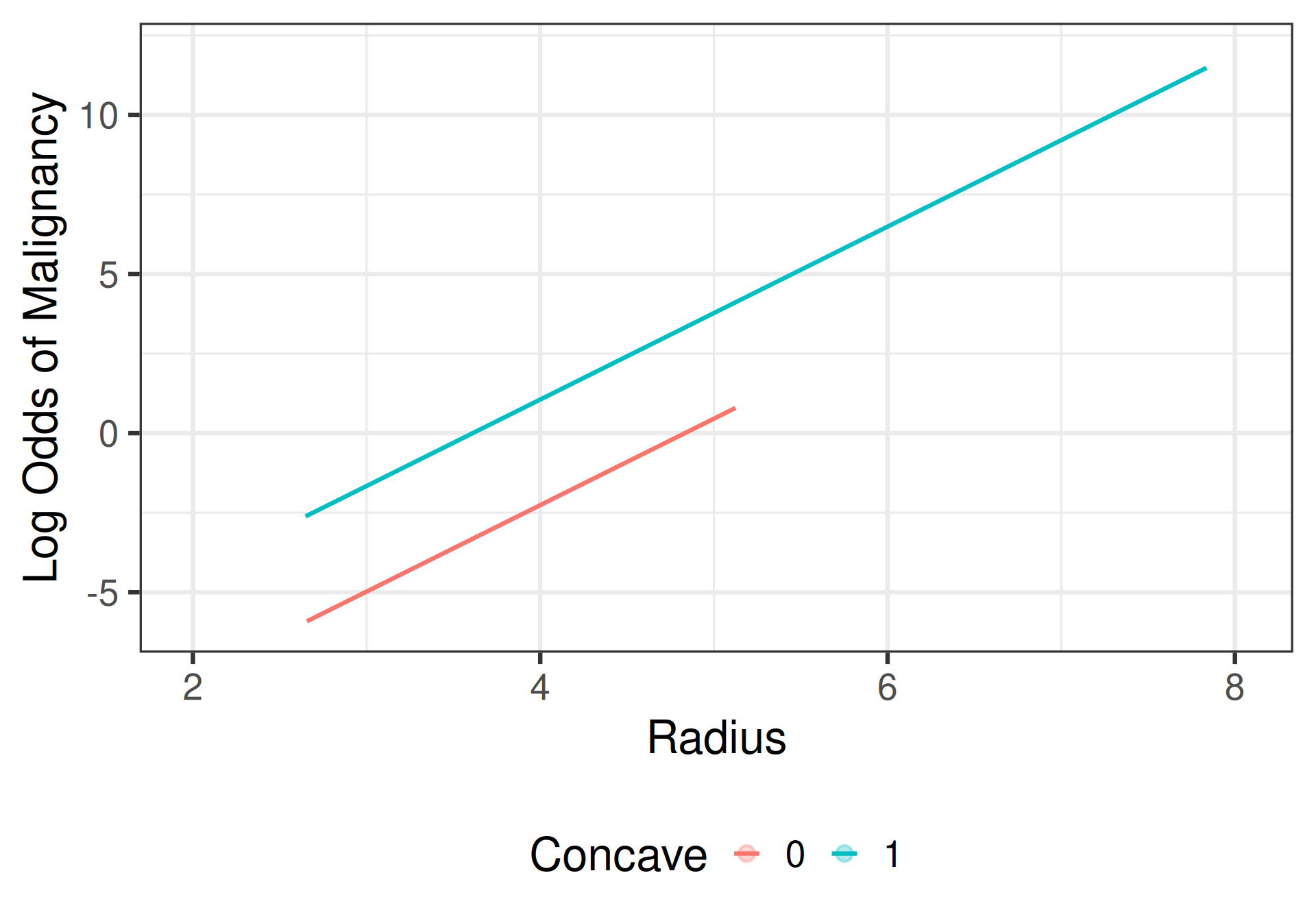
Visualizing the additive model

Additive Model

\[\begin{align*} \text{Convex Cells:} &\; \text{logit}\{\widehat{\pi}(\texttt{Radius},\texttt{Concave}= 0)\} = -13.132 + 2.718(\texttt{Radius}) \\ \text{Concave Cells:} &\; \text{logit}\{\widehat{\pi}(\texttt{Radius}, \texttt{Concave} = 1)\} = -9.813 + 2.718(\texttt{Radius}) \end{align*}\]

Interpretation: additive model

Additive model

\[ \text{logit}\left\{\widehat{\pi}(\texttt{Radius}, \texttt{Concave})\right\} = -13.132 + 2.718(\texttt{Radius}) + 3.319(\texttt{Concave}) \]

• Intercept: The estimated odds of malignancy among tumors with an average cell nuclei radius of 0 \(\mu\)m and convex nuclei is 0.000002.

\[\text{Scratch work: }e^{-13.132}\approx 0.000002\]

Interpretation: additive slopes

• Radius: Holding cell shape constant, each additional \(\mu\)m increase in the average radius of the cell nuclei is associated with a 15.15 times change (1,415% increase) in the odds of tumor malignancy.

\[\text{Scratch work: }e^{2.718} = 15.15 \implies (15.15-1)\times 100\% = 1415\%\]

• Concave: Among tumors with the same average cell radius, the odds that a tumor with concave cell nuclei is malignant are 27.63 times as great as (2,663% greater than) the odds when the cells are convex.

\[\text{Scratch work: }e^{3.319} = 27.63 \implies (27.63-1)\times 100\% = 2663\%\]

Interaction model for malignancy

If we want to allow the relationship between average cell radius (or cell shape) and \(\pi\) to differ depending on the other visual characteristic…

Population Model

\[\begin{align*} \text{logit}\{\pi(\texttt{Radius}, \texttt{Concave})\} = & \ \beta_0 + \beta_1(\texttt{Radius}) + \beta_2(\texttt{Concave}) \\ &+ \beta_3(\texttt{Radius})(\texttt{Concave}) \end{align*}\]

Fitted Model

\[\begin{align*} \text{logit}\{\widehat{\pi}(\texttt{Radius}, \texttt{Concave})\} = & \ -15.036 + 3.189(\texttt{Radius}) + 6.455(\texttt{Concave}) \\ &- 0.778(\texttt{Radius})(\texttt{Concave}) \end{align*}\]

Fitting the interaction model

interact_glm <- glm(
  Malignant ~ Radius * Concave, 
  data = cell, 
  family = "binomial"
)
summary(interact_glm)

Call:
glm(formula = Malignant ~ Radius * Concave, family = "binomial", 
    data = cell)

Coefficients:
               Estimate Std. Error z value Pr(>|z|)    
(Intercept)    -15.0357     2.4698  -6.088 1.14e-09 ***
Radius           3.1889     0.6050   5.271 1.36e-07 ***
Concave          6.4551     3.0460   2.119   0.0341 *  
Radius:Concave  -0.7784     0.7472  -1.042   0.2976    
---
Signif. codes:  0 '***' 0.001 '**' 0.01 '*' 0.05 '.' 0.1 ' ' 1

(Dispersion parameter for binomial family taken to be 1)

    Null deviance: 751.44  on 568  degrees of freedom
Residual deviance: 222.91  on 565  degrees of freedom
AIC: 230.91

Number of Fisher Scoring iterations: 7

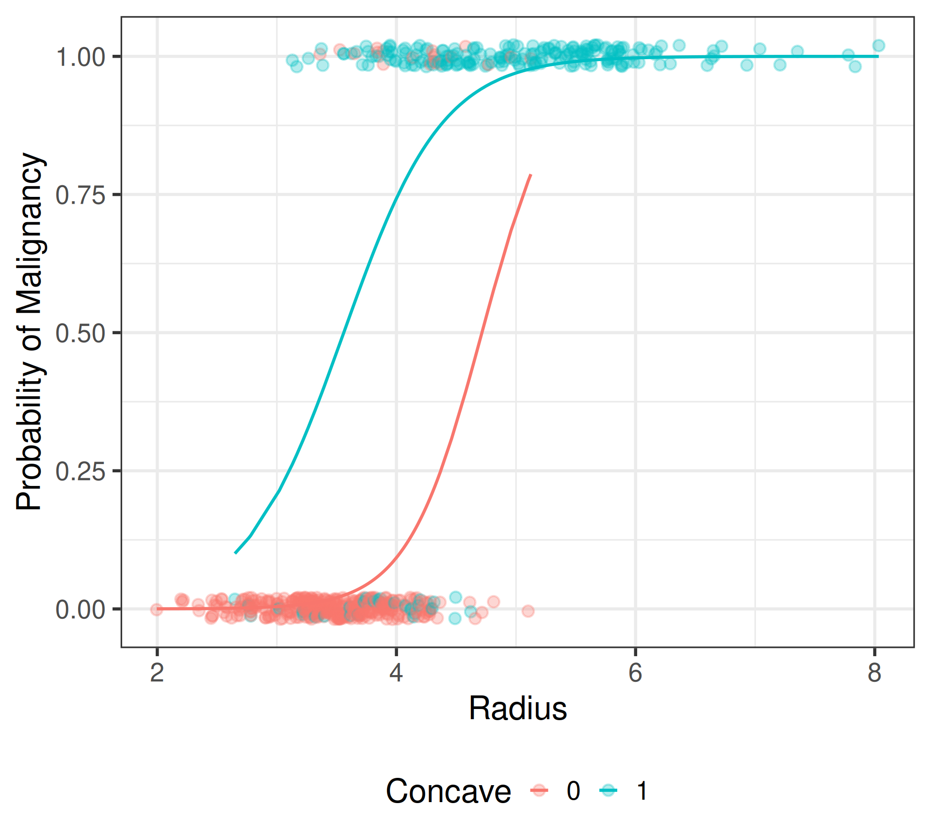
Visualizing interaction model

Interaction Model

\[\begin{align*} \text{Convex Cells:} &\; \text{logit}\{\widehat{\pi}(\texttt{Radius},\texttt{Concave} = 0)\} = -15.036 + 3.189(\texttt{Radius}) \\ \text{Concave Cells:} &\; \text{logit}\{\widehat{\pi}(\texttt{Radius}, \texttt{Concave} = 1)\} = -8.581 + 2.411(\texttt{Radius}) \end{align*}\]

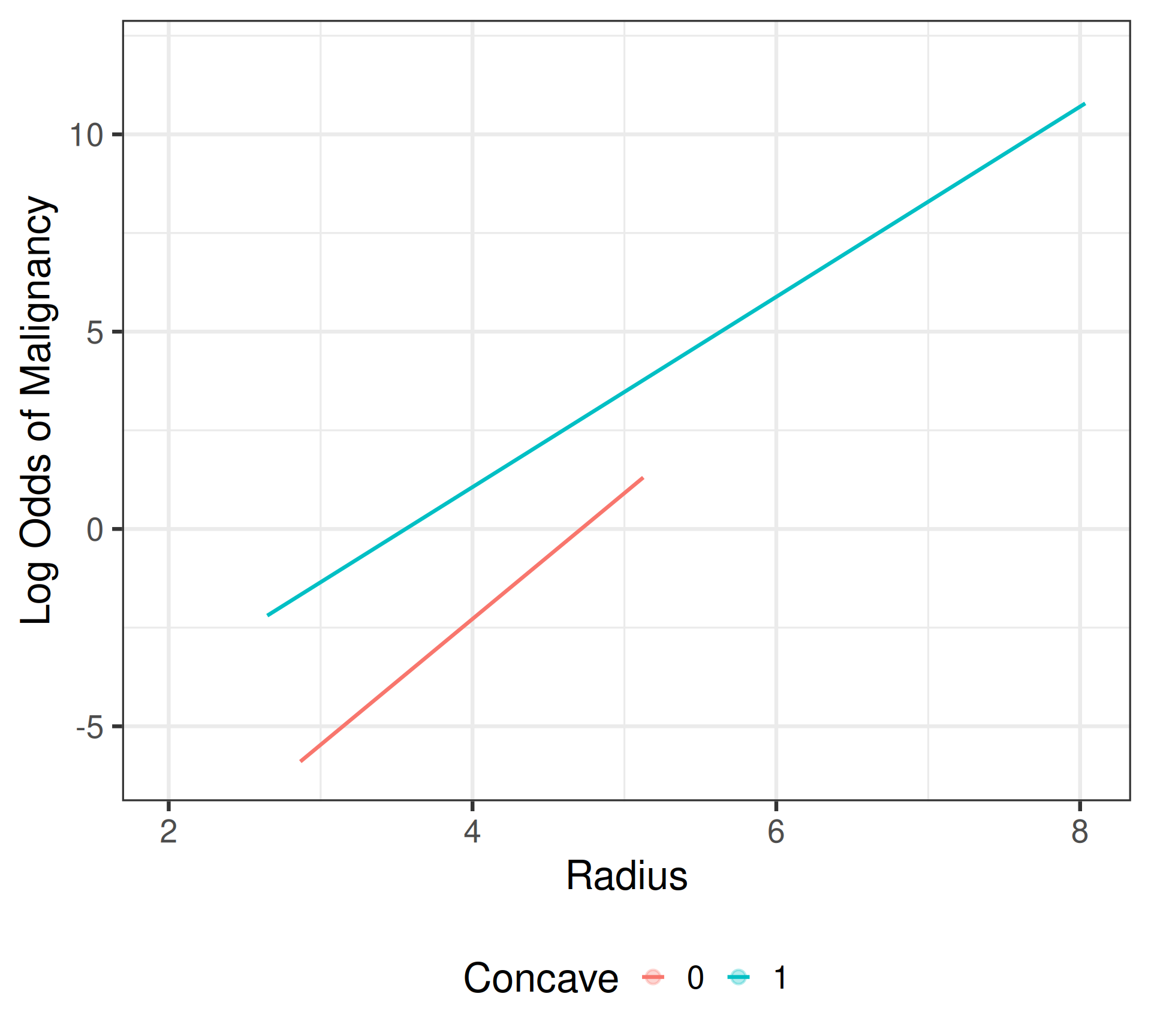
Interpretation: Radial size

Our interpretations now require us to specify at which value we are holding the other variable involved in the interaction constant:

Interaction Model

\[\begin{align*} \text{logit}\{\widehat{\pi}(\texttt{Radius}, \texttt{Concave})\} = & \ -15.036 + 3.189(\texttt{Radius}) + 6.455(\texttt{Concave}) \\ &- 0.778(\texttt{Radius})(\texttt{Concave}) \end{align*}\]

• Radius: For tumors with convex cell nuclei, each one \(\mu\)m increase in the average nuclei radius is associated with a 24.26 times change (2,326% increase) in the odds of tumor malignancy. \[\text{Scratch work: }e^{3.189} = 24.26 \implies (24.26-1)\times 100\% = 2326\%\]
• Radius: For tumors with concave cell nuclei, each one \(\mu\)m increase in the average nuclei radius is associated with a 11.15 times change (1,015% increase) in the odds of tumor malignancy. \[\text{Scratch work: }e^{3.189 - 0.778} = 11.15 \implies (11.15-1)\times 100\% = 1015\%\]

Interpretation: Concavity

• Concave: For tumors with an average nuclei radius of 4 \(\mu\)m, the odds of malignancy are 28.30 times as high (2,730% higher) when the cell nuclei are concave as they are when the cell nuclei are convex. \[\text{Scratch work: }e^{6.455 - 0.778(4)} = 28.30 \implies (28.30-1)\times 100\% = 2730\%\]
• Concave: For tumors with an average nuclei radius of 7 \(\mu\)m, the odds of malignancy are 2.74 times as high (174% higher) when the cell nuclei are concave as they are when the cell nuclei are convex. \[\text{Scratch work: }e^{6.455 - 0.778(7)} = 2.74 \implies (2,74-1)\times 100\% = 174\%\]

Model fit

# Iterate glance() over both models and combine
list(additive_glm, interact_glm) |>
  map(glance) |>
  bind_rows()

# A tibble: 2 × 8
  null.deviance df.null logLik   AIC   BIC deviance df.residual  nobs
          <dbl>   <int>  <dbl> <dbl> <dbl>    <dbl>       <int> <int>
1          751.     568  -112.  230.  243.     224.         566   569
2          751.     568  -111.  231.  248.     223.         565   569

# Comparing the models using a likelihood ratio test
anova(additive_glm, interact_glm, test = "Chisq")

Analysis of Deviance Table

Model 1: Malignant ~ Radius + Concave
Model 2: Malignant ~ Radius * Concave
  Resid. Df Resid. Dev Df Deviance Pr(>Chi)
1       566     224.02                     
2       565     222.91  1   1.1039   0.2934

Classification

Related questions

1. Prediction: What is the probability that a person with an average cell radius of 5\(\mu\)m and convex cell nuclei has a malignant tumor?
2. Classification: Can we use these probabilities to determine who actually does and does not have a malignant tumor?

Calculating Predicted Probabilities

Research Question

What is the probability that a person with an average cell radius of 5 \(\mu\)m and convex cell nuclei has a malignant tumor?

\[\widehat{\pi}(5, 0) = \frac{e^{-13.132 + 2.718(5) + 3.319(0)}}{1 + e^{-13.132 + 2.718(5) + 3.319(0)}} = 0.612\]

patient_subpopulation <- data.frame(Radius = 5, Concave = 0)
additive_glm |> 
  augment(newdata = patient_subpopulation, type.predict = "response")

# A tibble: 1 × 3
  Radius Concave .fitted
   <dbl>   <dbl>   <dbl>
1      5       0   0.612

CIs for Predicted Odds

Research Question

What is the probability that a person with an average cell radius of 5 \(\mu\)m and convex cell nuclei has a malignant tumor?

\[\begin{align*} \text{logit}(\hat{\pi}) &\pm z^* \cdot SE_{\text{logit}(\hat{\pi})} \\ 0.456 &\pm 1.96 \cdot 0.442 = (-0.410, 1.322) \end{align*}\]

additive_glm |> 
  augment(
    newdata = patient_subpopulation,
    type.predict = "link", se_fit = TRUE
  )

# A tibble: 1 × 4
  Radius Concave .fitted .se.fit
   <dbl>   <dbl>   <dbl>   <dbl>
1      5       0   0.456   0.442

CIs for Predicted Probabilities

• First build them for the log odds: \[ 0.456 \pm (1.96)(0.442) = (-0.410, 1.322) \]
• Then transform both endpoints back to probability scale: \[ \left(\frac{e^{-0.410}}{1 + e^{-0.410}}, \ \frac{e^{1.322}}{1 + e^{1.322}}\right) = (0.399, 0.790) \]

# do it manually!
c(exp(-0.410) / (1 + exp(-0.410)), exp(1.322) / (1 + exp(1.322)))

[1] 0.3989121 0.7895143

# write a function!
logit <- function(x) exp(x) / (1 + exp(x))
logit(c(-0.410, 1.322))

[1] 0.3989121 0.7895143

Answers

• Prediction: What is the probability that a person with an average cell radius of 5 \(\mu\)m and convex cell nuclei has a malignant tumor?
  • We estimate this probability to be 61.2%.
  • We are 95% confident that the true probability that an individual with an average cell radius of 5 \(\mu\)m and convex cell nuclei has a malignant tumor is between 39.9% and 70.0%.
• Classification: Can we use these probabilities to determine who actually does and does not have malignant cancer?
  • How well did our model do at making these predictions?
  • If all we had to go off of was the predicted probability \(\widehat{\pi}\), could we reliably figure out who actually has a malignant tumor?

Classification with logistic regression

Intuition

Model does a good job at predicting tumor malignancy if it assigns higher values of \(\widehat{\pi}\) to people who actually have malignant tumors and lower values of \(\widehat{\pi}\) to people who do not

• A new patient comes along whose true tumor status we don’t know, but whose predicted probability is \(\widehat{\pi} = 0.612\)
• Should we refer this patient for surgery?

Consider two models

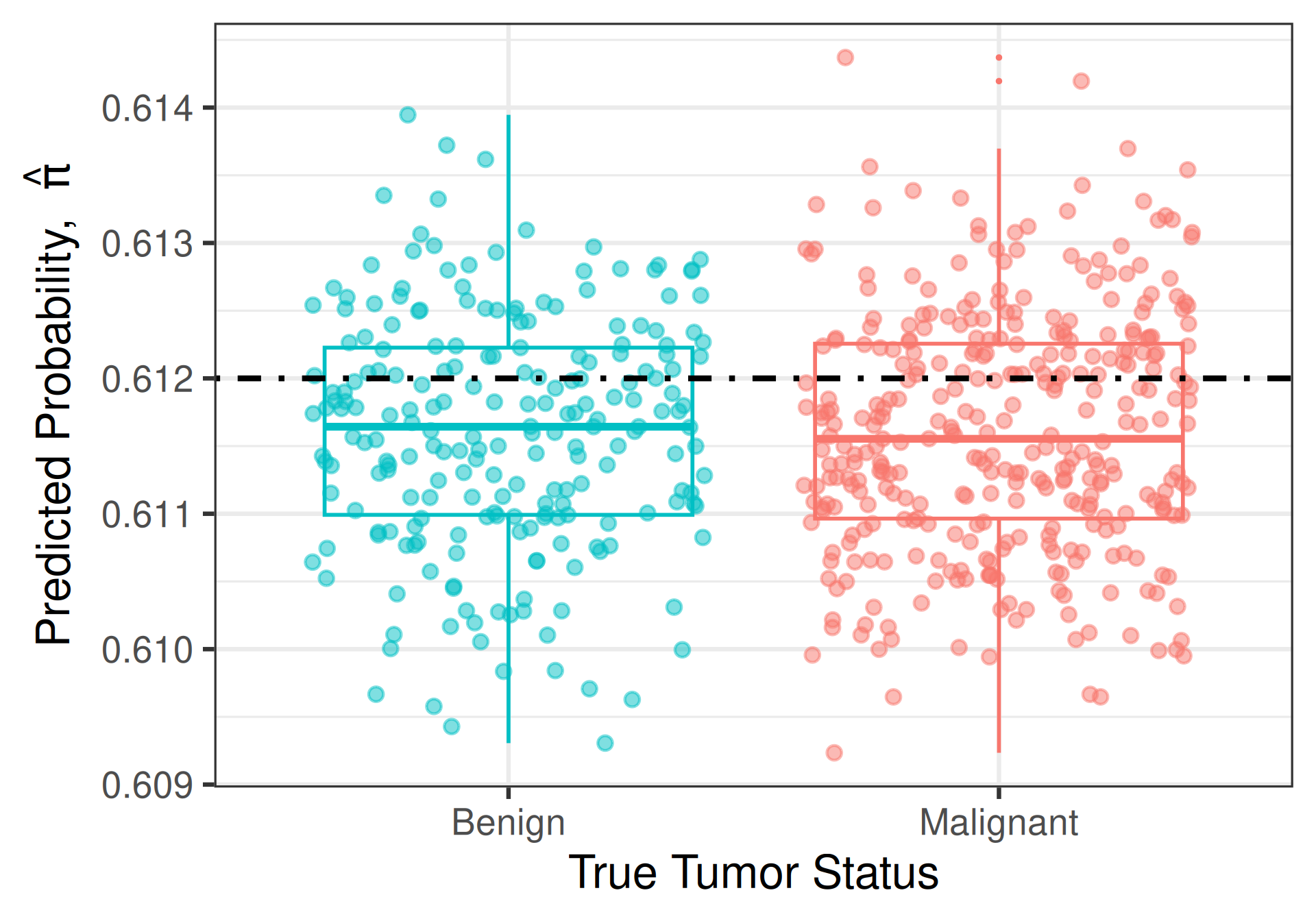
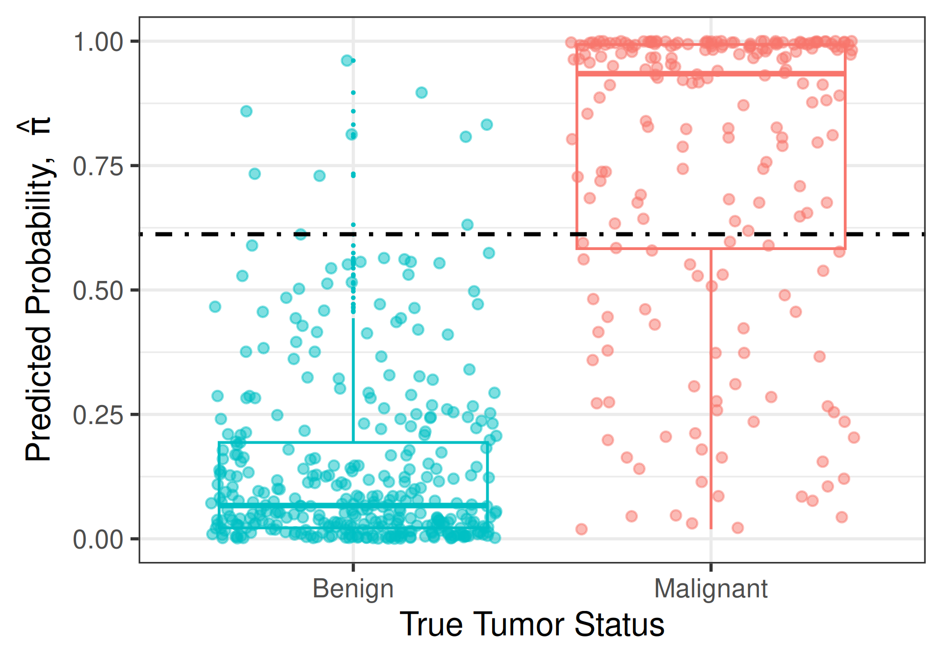
Classification Cut-Offs

• Set a cut-off: \(\pi_0 = 0.5\)

\[\begin{alignat*}{2} &\widehat{\pi} > 0.5 \quad &&\implies \quad \text{classify as a "malignant" tumor, }\widehat{y} = 1 \\ &\widehat{\pi} \leq 0.5 \quad &&\implies \quad \text{classify as a "benign" tumor, }\widehat{y} = 0 \\ \end{alignat*}\]

p_hat <- additive_glm |> 
  augment(type.predict = "response") |>
  mutate(
    y = factor(Malignant, levels = c(0, 1), labels = c("Benign", "Malignant")),
    pred = factor(ifelse(.fitted > 0.5, "Malignant", "Benign"))
  )
p_hat |>
  sample_n(4) |>
  select(.fitted, pred, Malignant)

# A tibble: 4 × 3
  .fitted pred   Malignant
    <dbl> <fct>      <dbl>
1  0.0125 Benign         0
2  0.0265 Benign         0
3  0.0276 Benign         0
4  0.0173 Benign         0

Classification tables

Any classification is either correct or incorrect:

p_hat |>
  select(Malignant, pred) |>
  table() |>
  addmargins()

         pred
Malignant Benign Malignant Sum
      0      335        22 357
      1       24       188 212
      Sum    359       210 569

Tip

Believe it or not, these tables are called confusion matrices!

Classification metrics

• Sensitivity: the proportion of true successes that we correctly classify as a “success” \[\begin{equation*} \text{sens} = \frac{\#\text{ correctly predicted malignant}}{\#\text{ with malignant tumors}} = \frac{TP}{TP + FN} \end{equation*}\]
• Specificity: the proportion of true failures that we correctly classify as a “failure” \[\begin{equation*} \text{spec} = \frac{\#\text{ correctly predicted benign}}{\#\text{ with benign tumors}} = \frac{TN}{FP + TN} \end{equation*}\]

Try \(\pi_0 = 0.5\)

# A tibble: 3 × 3
  .metric  .estimator .estimate
  <chr>    <chr>          <dbl>
1 accuracy binary         0.919
2 sens     binary         0.938
3 spec     binary         0.887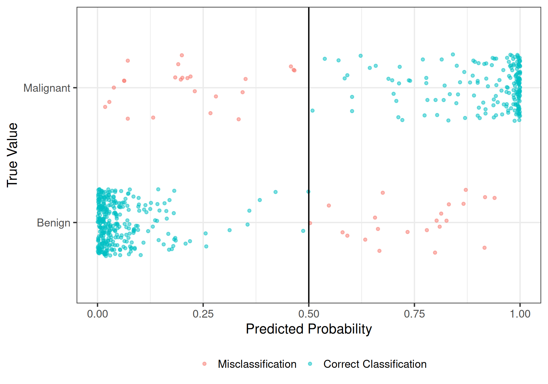

Try \(\pi_0 = 0.05\)

# A tibble: 3 × 3
  .metric  .estimator .estimate
  <chr>    <chr>          <dbl>
1 accuracy binary         0.789
2 sens     binary         0.672
3 spec     binary         0.986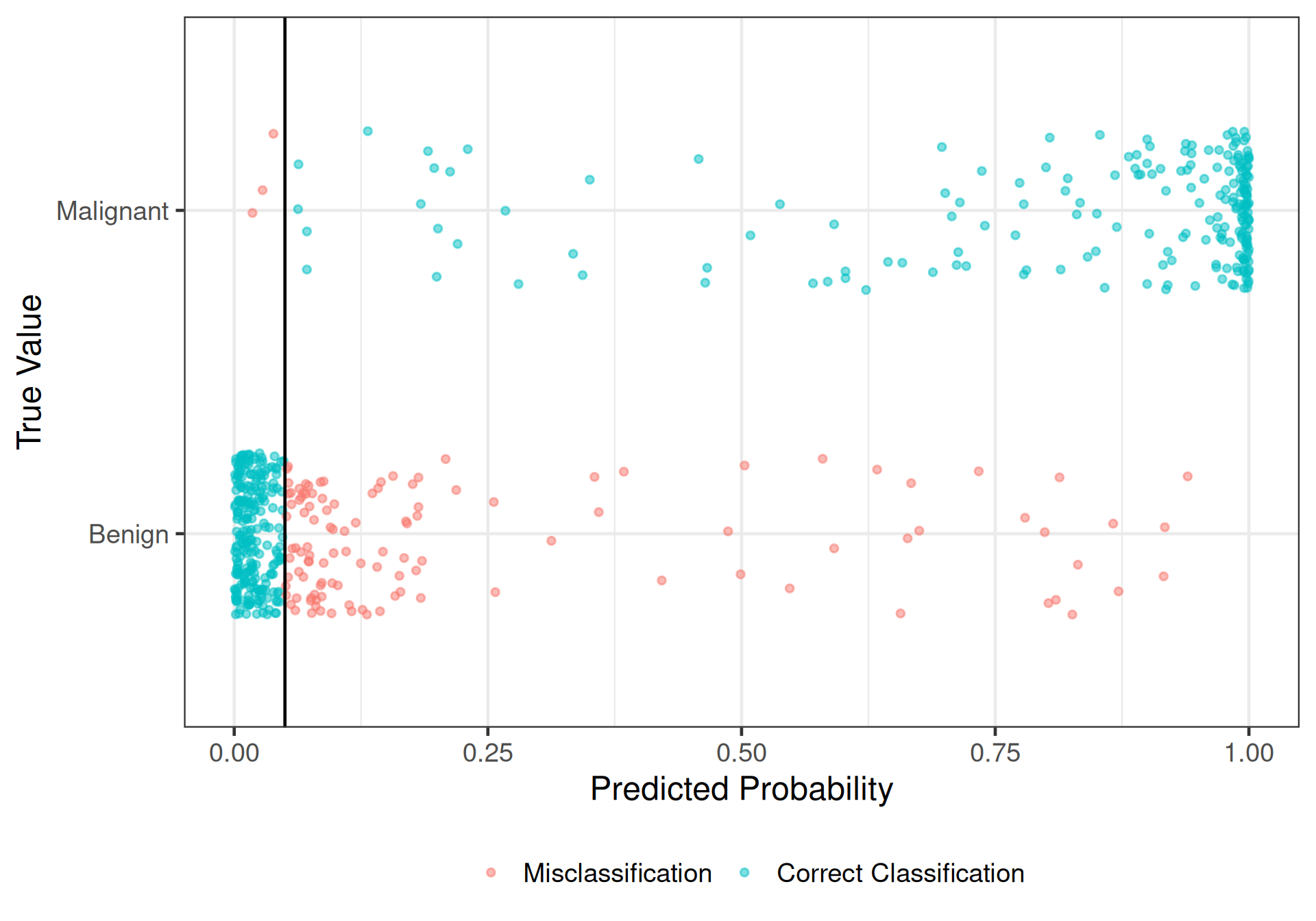

Try \(\pi_0 = 0.9\)

# A tibble: 3 × 3
  .metric  .estimator .estimate
  <chr>    <chr>          <dbl>
1 accuracy binary         0.870
2 sens     binary         0.992
3 spec     binary         0.665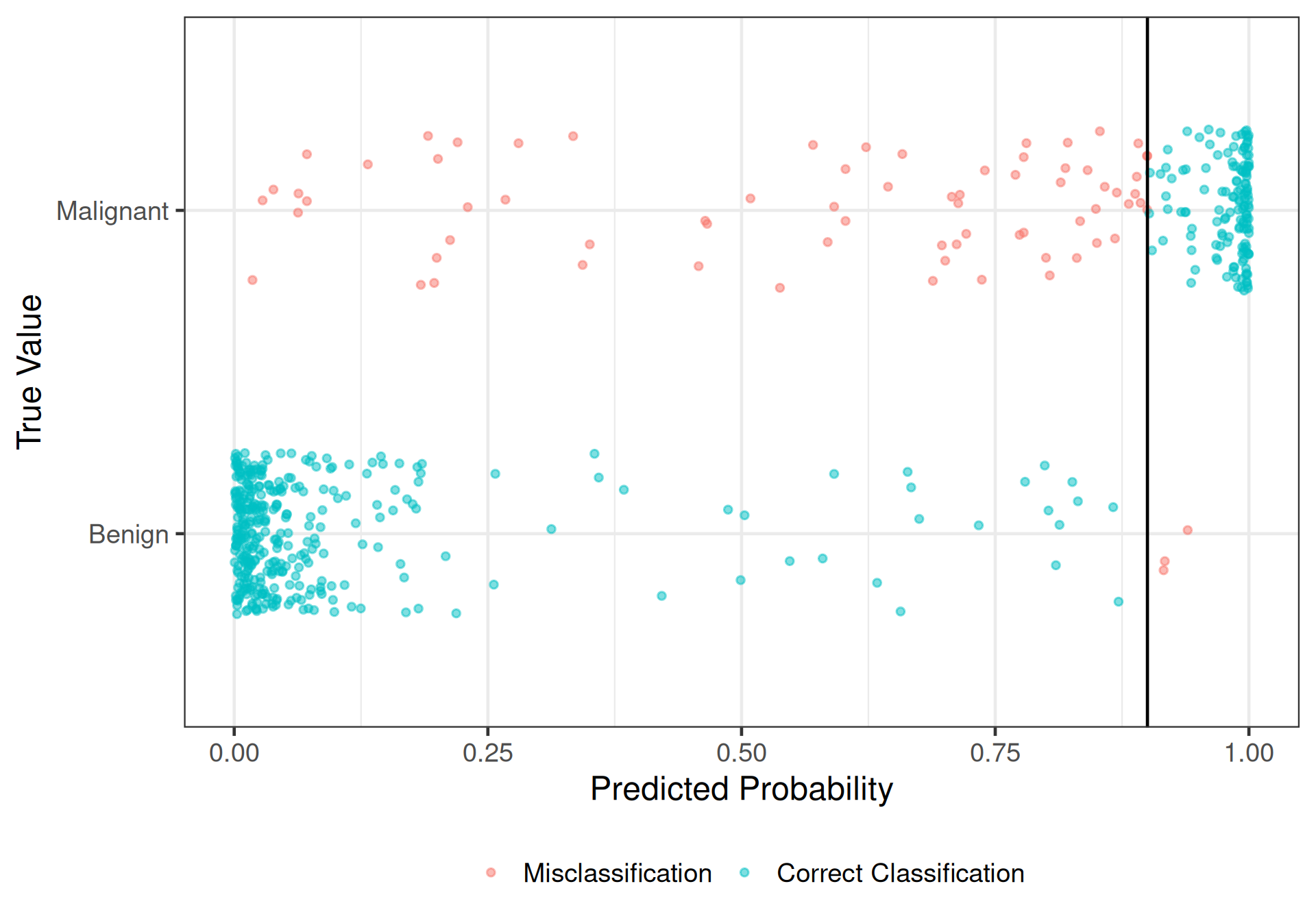

Trade-offs

• A model with high discrimination makes it easier to find a cut-off that produces a good balance between sensitivity and specificity

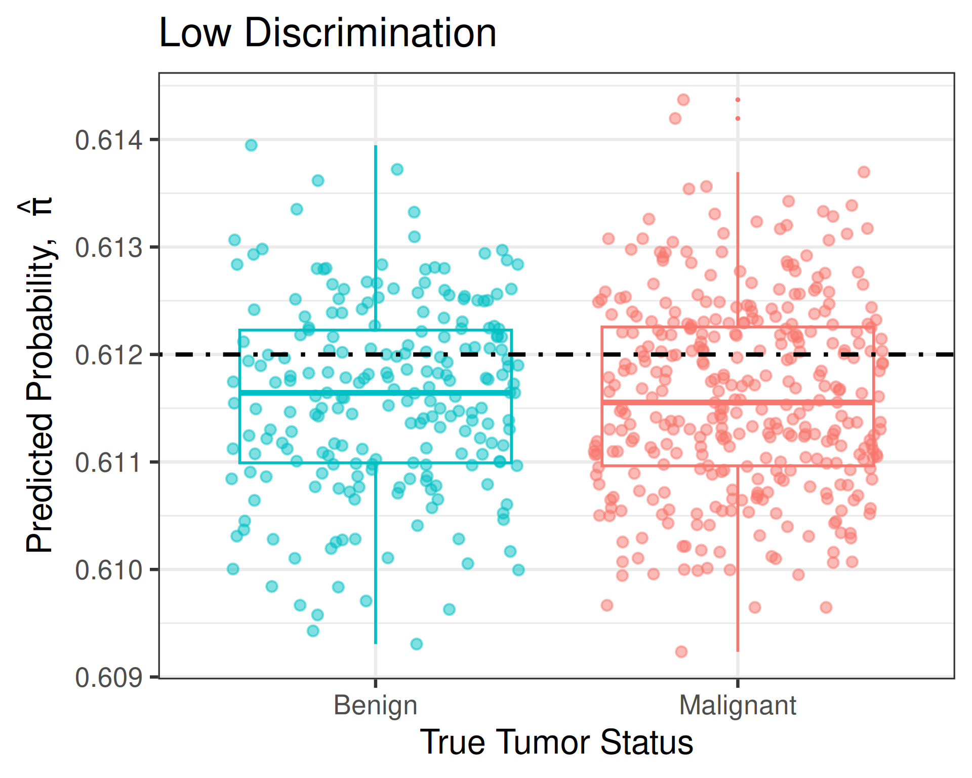
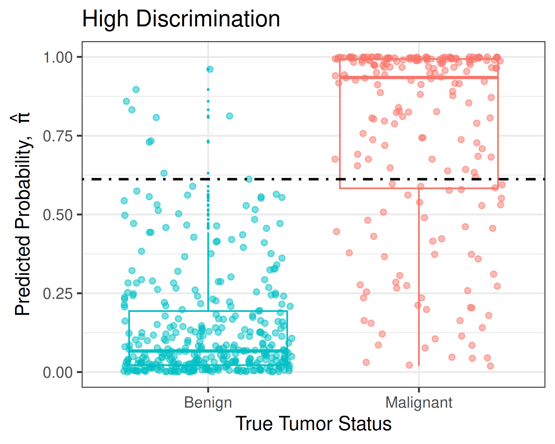
ROC curve

Receiver Operating Characteristic: Visualizes the trade-off between sensitivity and specificity across a range of cut-offs

library(yardstick)
p_hat |>
  roc_curve(truth = y, .fitted, event_level = "second") |>
  autoplot()

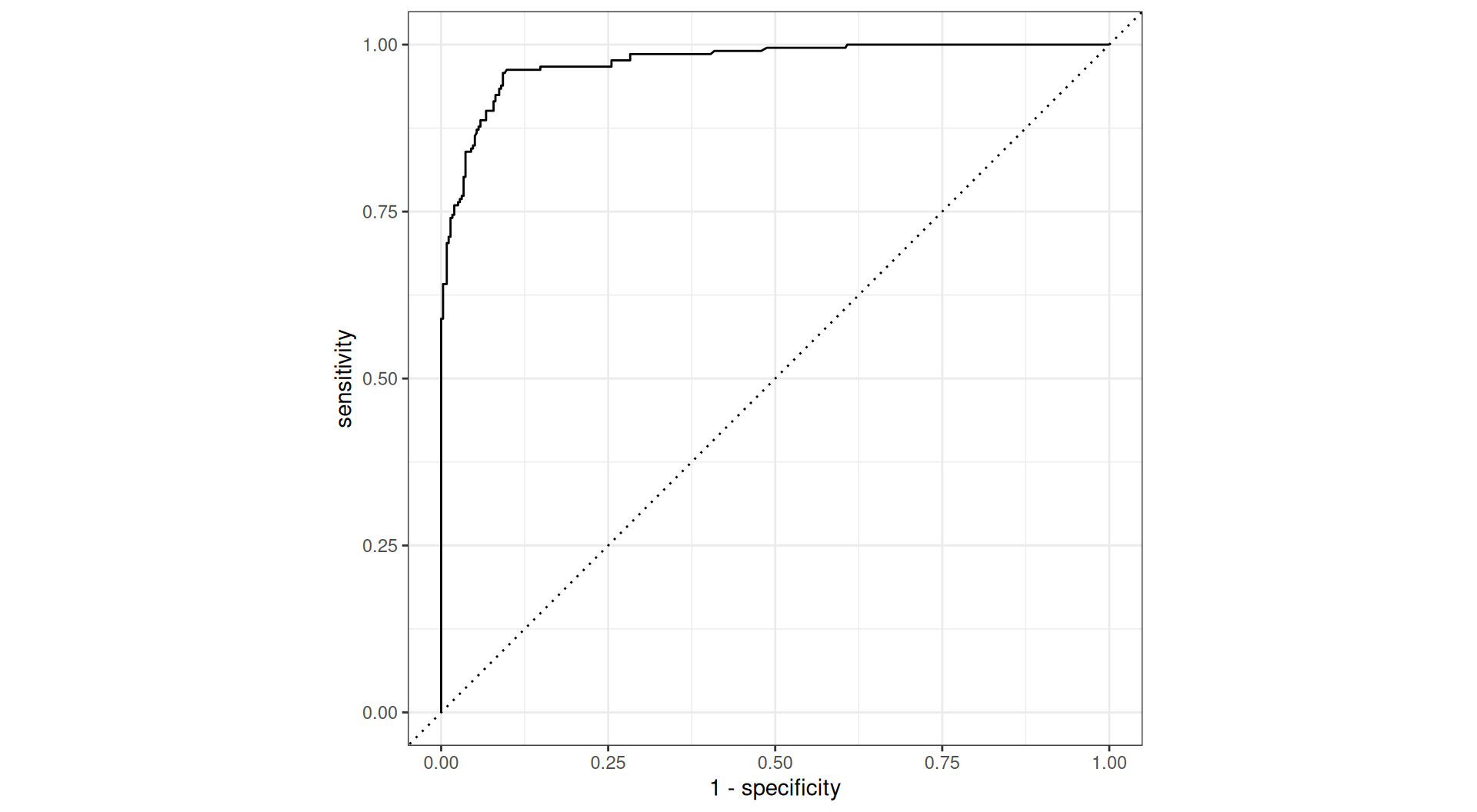
Area under the ROC curve (AUC)

• single number summarizing the overall discrimination
  • a.k.a., the c-statistic or concordance index
• If we randomly select one success and one failure, what are the chances that the true success has a higher predicted probability than the true failure?

p_hat |>
  roc_auc(truth = y, .fitted, event_level = "second")

# A tibble: 1 × 3
  .metric .estimator .estimate
  <chr>   <chr>          <dbl>
1 roc_auc binary         0.974

Note

• Would you prefer a larger or smaller AUC?
• What would the AUC be if the ROC curve fell exactly on the \(y=x\) line?

Extreme ROC curves

Perfect Discrim.: \(AUC = 1\)

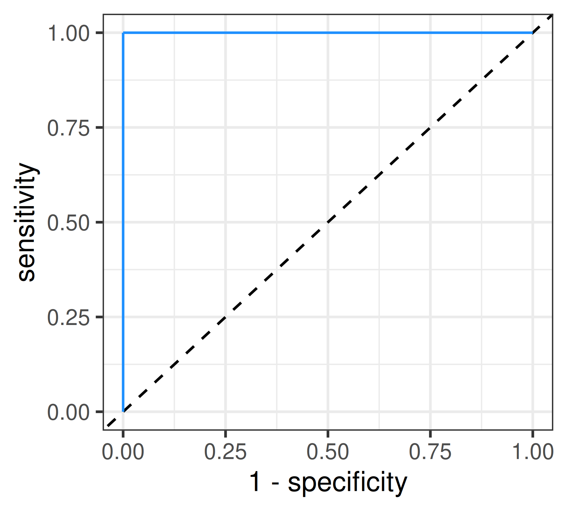
Random Guessing: \(AUC = 0.5\)

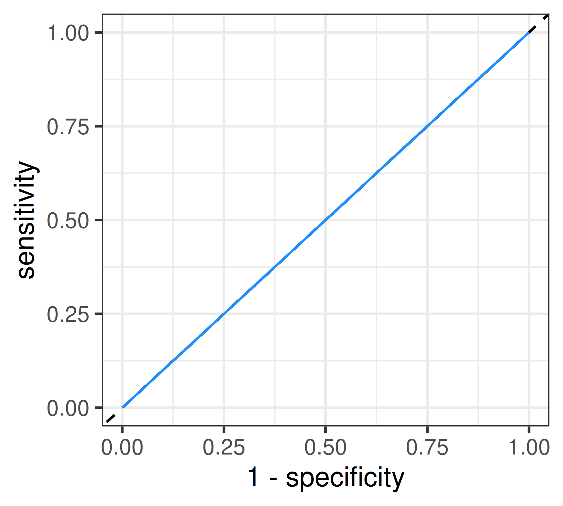
Data Coding Error?: \(AUC = 0\)

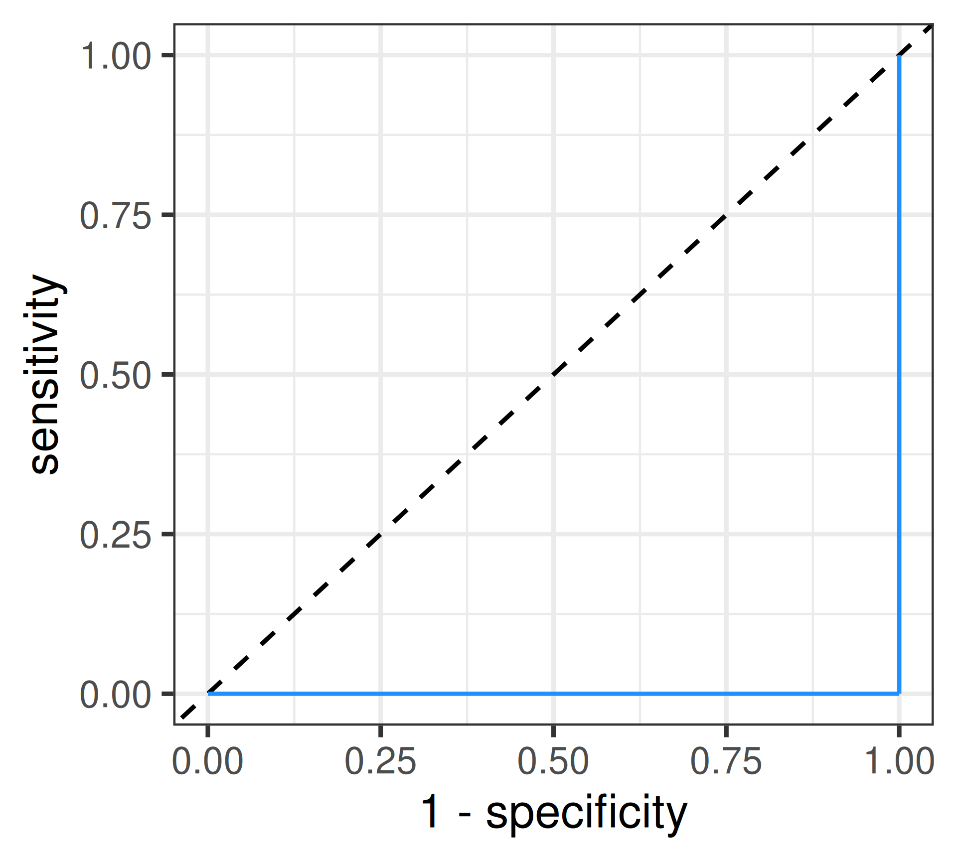
Selecting a classification cut-off (\(\pi_0\))

• Different choices of \(\pi_0\) will navigate the trade-off between sensitivity and specificity differently
• Desirable \(\pi_0\) is thus context-dependent:
  • If we want to minimize the chance we miss actual malignant tumors, we want high sensitivity \(\iff\) select a lower cut-off for \(\pi_0\)
  • If we want to minimize the chance we mistakenly diagnose benign tumors as malignant, we want high specificity \(\iff\) select a higher cut-off for \(\pi_0\)

• If we value both metrics equally, another option is to maximize the vertical distance to the reference \(y = x\) line (called Youden’s index): \[\max\left\{\text{sensitivity} + \text{specificity} - 1\right\}\]

j_index(p_hat, truth = y, estimate = pred, event_level = "second")

# A tibble: 1 × 3
  .metric .estimator .estimate
  <chr>   <chr>          <dbl>
1 j_index binary         0.825