25-Conditions for Logistic Regression

SDS 291

Prof. Baumer

December 3, 2025

Conditions for Logistic Regression

  • Randomness: Was the data generated by a random process?
  • Independence: Do the observational units behave independently? Or do they depend on each other in some meaningful way?
  • Linearity: Is the relationship between the explanatory variable and the empirical logits of the response variable linear?

Empirical logits

  • Empirical: based on the observed data
  • Empirical logit: the estimated log odds of success, based only on the observed sample proportions (and not the model)
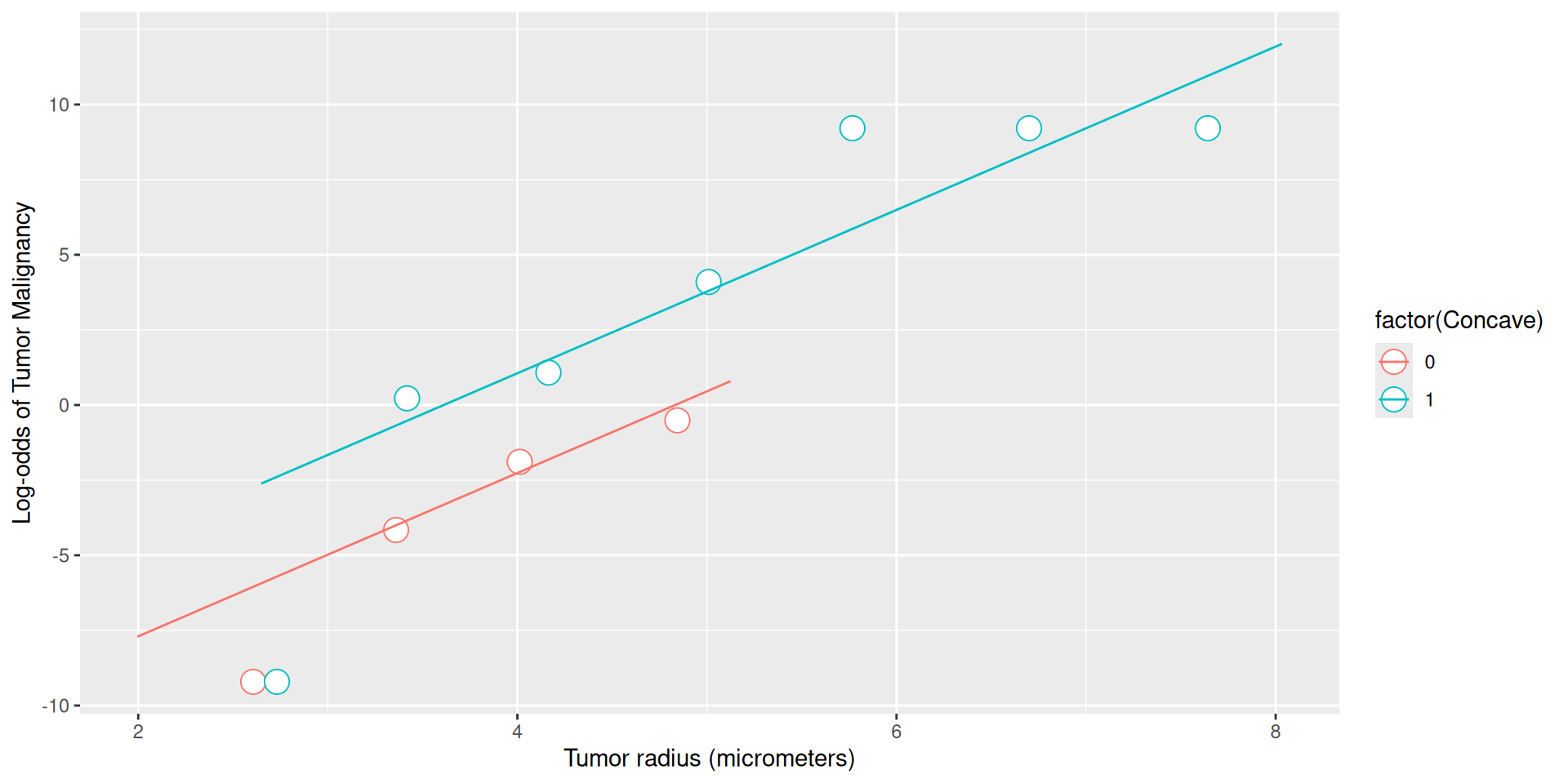
  • Empirical logit plot: tool for evaluating whether the log odds of success have a linear relationship with \(x\)

Ex: additive model for tumors

mod_tumor <- glm(Malignant ~ Radius + Concave, data = cell, family = "binomial")
summary(mod_tumor)

Call:
glm(formula = Malignant ~ Radius + Concave, family = "binomial", 
    data = cell)

Coefficients:
            Estimate Std. Error z value Pr(>|z|)    
(Intercept) -13.1320     1.4932  -8.795  < 2e-16 ***
Radius        2.7175     0.3663   7.418 1.19e-13 ***
Concave       3.3192     0.3545   9.362  < 2e-16 ***
---
Signif. codes:  0 '***' 0.001 '**' 0.01 '*' 0.05 '.' 0.1 ' ' 1

(Dispersion parameter for binomial family taken to be 1)

    Null deviance: 751.44  on 568  degrees of freedom
Residual deviance: 224.02  on 566  degrees of freedom
AIC: 230.02

Number of Fisher Scoring iterations: 7

Set up the spaces

data_space <- cell |>
  ggplot(aes(x = Radius, y = Malignant, color = factor(Concave))) +
  geom_jitter(height = 0.02, alpha = 0.5) +
  scale_y_continuous("Probability of Tumor Malignancy") +
  scale_x_continuous("Tumor radius (micrometers)")
tumors_aug <- mod_tumor |>
  broom::augment() |>
  mutate(
    odds_hat = exp(.fitted),
    p_hat = odds_hat / (1 + odds_hat)
  )

model_space <- data_space +
  geom_point(data = tumors_aug, aes(y = p_hat), shape = 1) +
  geom_smooth(
    method = "glm", 
    method.args = list(family = binomial), 
    se = FALSE
  )

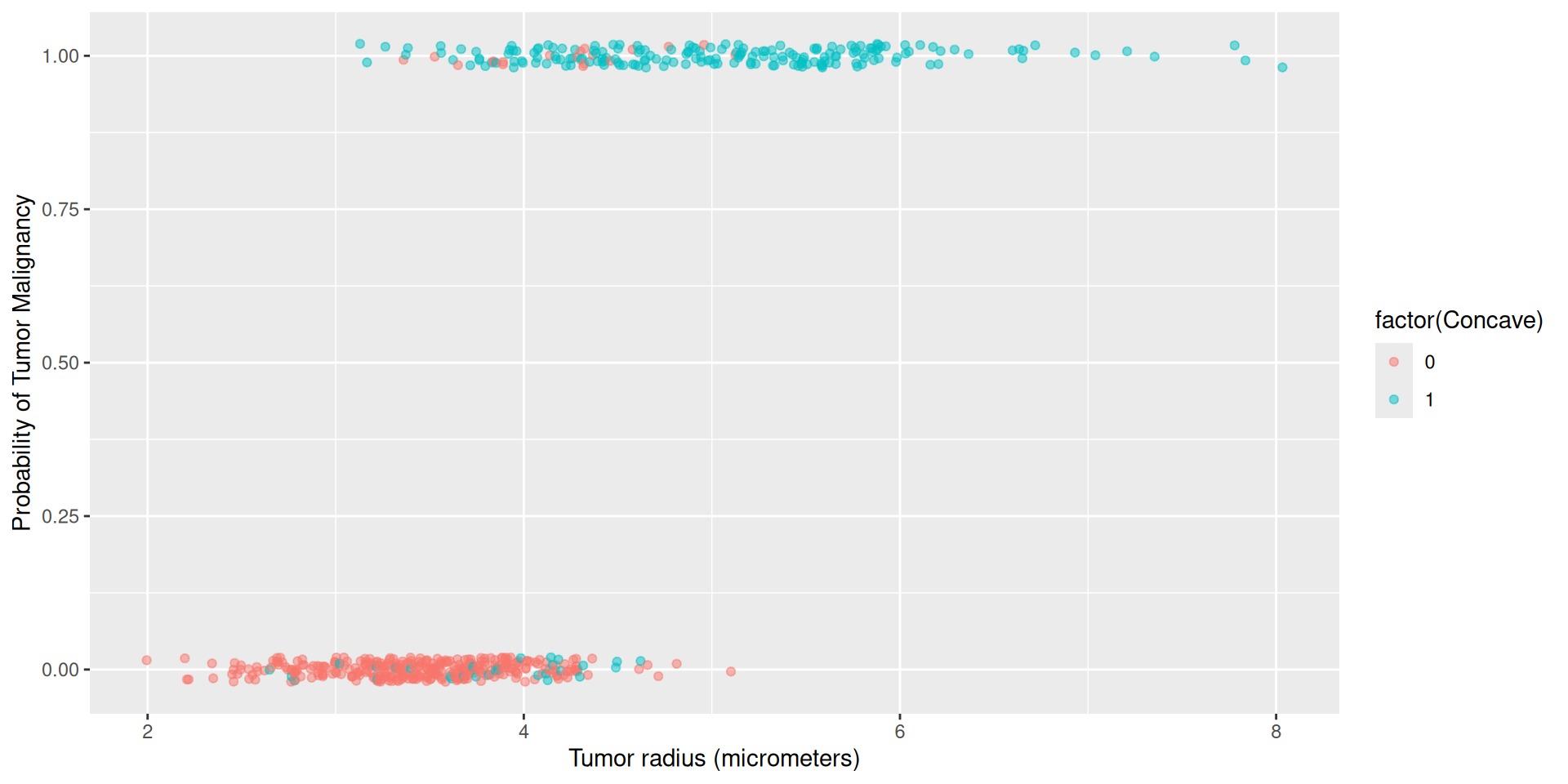
Visualize the data space

data_space

Visualize the model in the data space!
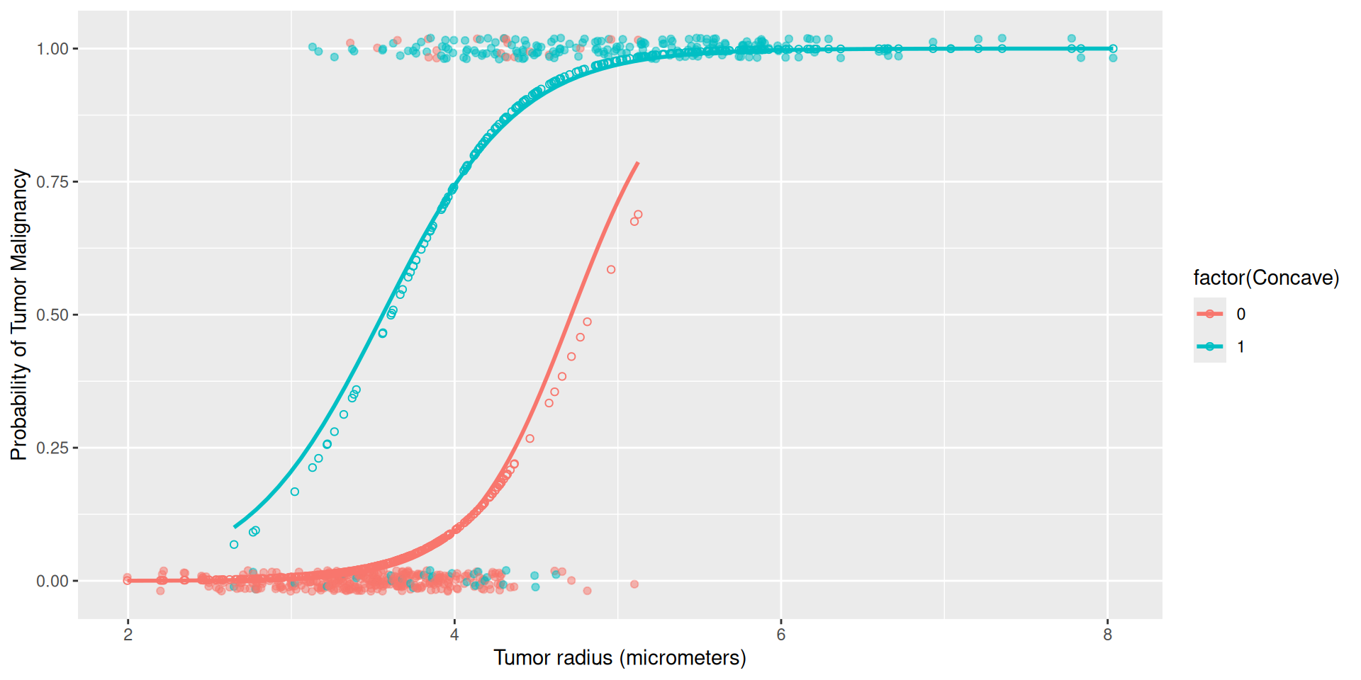
model_space

Compute \(\bar{y}\) for bins of \(x\)

cell_binned <- cell |>
  group_by(
    radius_bin = cut(Radius, breaks = 7), 
    Concave
  ) |>
  summarize(
    n = n(),
    radius_coord = mean(Radius),
    malignant_prop = mean(Malignant)
  )
cell_binned
# A tibble: 11 × 5
# Groups:   radius_bin [7]
   radius_bin  Concave     n radius_coord malignant_prop
   <fct>         <dbl> <int>        <dbl>          <dbl>
 1 (1.99,2.86]       0    44         2.61         0     
 2 (1.99,2.86]       1     3         2.73         0     
 3 (2.86,3.72]       0   195         3.36         0.0154
 4 (2.86,3.72]       1    18         3.42         0.556 
 5 (3.72,4.58]       0    99         4.01         0.131 
 6 (3.72,4.58]       1    71         4.16         0.746 
 7 (4.58,5.45]       0     8         4.84         0.375 
 8 (4.58,5.45]       1    61         5.01         0.984 
 9 (5.45,6.31]       1    57         5.77         1     
10 (6.31,7.17]       1     8         6.70         1     
11 (7.17,8.04]       1     5         7.64         1     

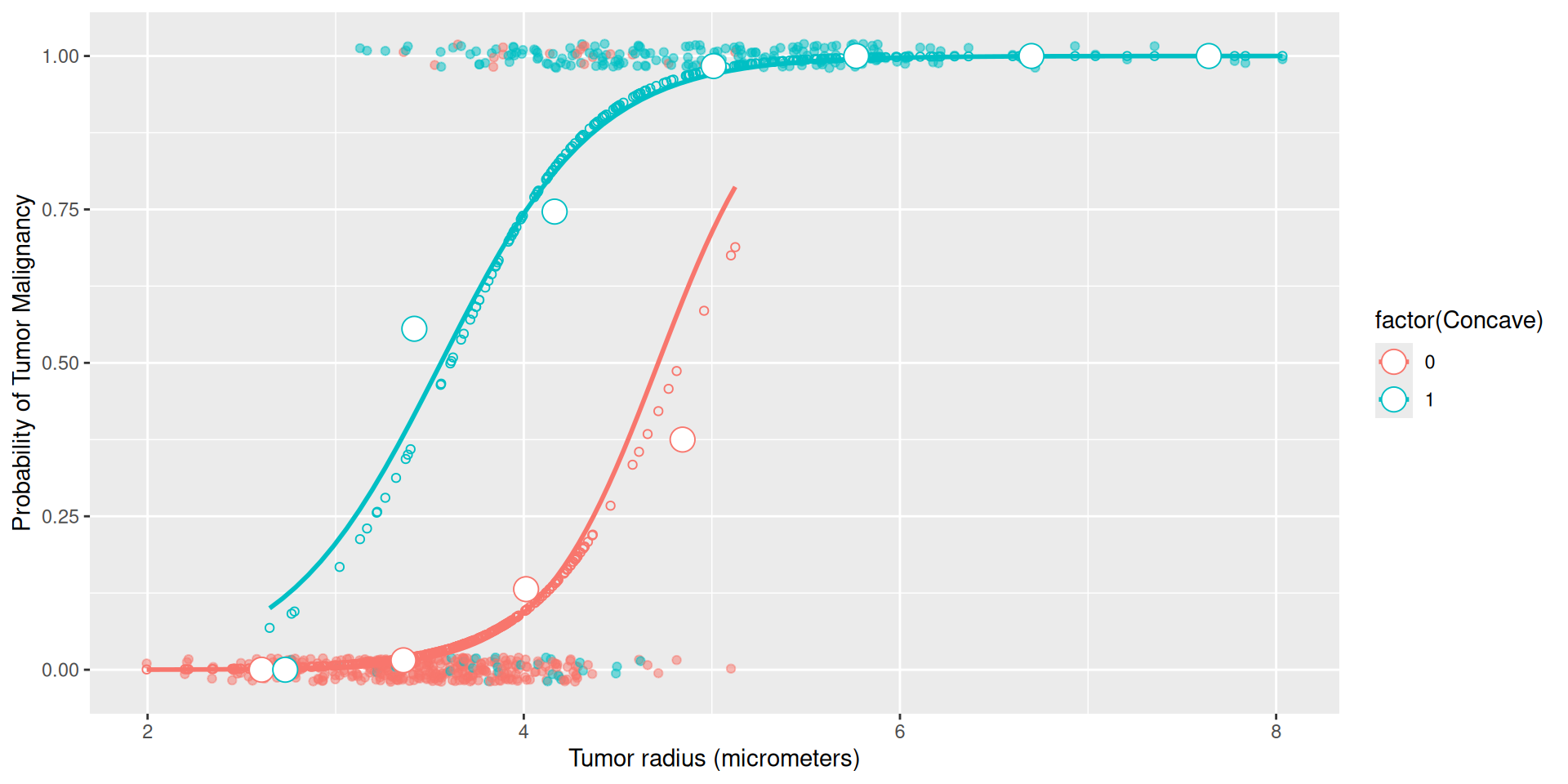
Add empirical means

model_space +
  geom_point(
    data = cell_binned, 
    aes(x = radius_coord, y = malignant_prop), 
    size = 5, shape = 21, fill = "white"
  )

Aside: why doesn’t this work?

data_space +
  scale_y_continuous(transform = "logit")
Scale for y is already present.
Adding another scale for y, which will replace the existing scale.
Warning in scale_y_continuous(transform = "logit"): prob-logis transformation
introduced infinite values.
Warning in min(x): no non-missing arguments to min; returning Inf
Warning in max(x): no non-missing arguments to max; returning -Inf
Warning: Position guide is perpendicular to the intended axis.
ℹ Did you mean to specify a different guide `position`?
Aside: edge behavior of logit function

Aside: define padded logit

logit_safe <- function(p) {
  max_p <- 0.9999
  p <- ifelse(p == 1, max_p, p)
  p <- ifelse(p == 0, 1 - max_p, p)
  log(p / (1 - p))
}
cell_binned <- cell_binned |>
  mutate(logit_malig_prop = logit_safe(malignant_prop))
cell_binned
# A tibble: 11 × 6
# Groups:   radius_bin [7]
   radius_bin  Concave     n radius_coord malignant_prop logit_malig_prop
   <fct>         <dbl> <int>        <dbl>          <dbl>            <dbl>
 1 (1.99,2.86]       0    44         2.61         0                -9.21 
 2 (1.99,2.86]       1     3         2.73         0                -9.21 
 3 (2.86,3.72]       0   195         3.36         0.0154           -4.16 
 4 (2.86,3.72]       1    18         3.42         0.556             0.223
 5 (3.72,4.58]       0    99         4.01         0.131            -1.89 
 6 (3.72,4.58]       1    71         4.16         0.746             1.08 
 7 (4.58,5.45]       0     8         4.84         0.375            -0.511
 8 (4.58,5.45]       1    61         5.01         0.984             4.09 
 9 (5.45,6.31]       1    57         5.77         1                 9.21 
10 (6.31,7.17]       1     8         6.70         1                 9.21 
11 (7.17,8.04]       1     5         7.64         1                 9.21 

Build tumor empirical logit plot

tumor_elp <- cell_binned |>
  ggplot(
    aes(x = radius_coord, y = logit_malig_prop, color = factor(Concave))
  ) +
  geom_point(size = 5, shape = 21, fill = "white") +
  geom_line(data = tumors_aug, aes(x = Radius, y = .fitted)) +
  scale_x_continuous("Tumor radius (micrometers)") +
  scale_y_continuous("Log-odds of Tumor Malignancy")

Visualize tumor empirical logit plot

tumor_elp