   inning team  retroID count      pitches                      play
1       1    1 vottj001     0         11>C                       SB2
2       1    1 vottj001    22 11>C.SB2>FBC                         K
3       3    1 vottj001    32       BBBCFC                         K
4       5    1 vottj001     0       1311>X S8/G6+.3-H;1-H;B-2(E5/TH)
5       7    1 vottj001    22        CBBCX                63/G6M.2-3
6      10    1 vottj001     0         <NA>                        NP
7      10    1 vottj001     0         <NA>                        NP
8      10    1 vottj001     0         <NA>                        NP
9      10    1 vottj001     0         <NA>                        NP
10 10 1 vottj001 32 ....BCFFBBC KLinear Weights
SDS 355
Prof. Baumer
September 15, 2025
What is the value of a play?
Watch
What happened?
- 1st and 3rd, nobody out
- Joey Votto singles
- Billy Hamilton scores from first!
- error allows Votto to advance to 2nd
- two actual runs scored
Retrosheet data
How valuable is a single?
- In this case, 2 runs scored, 2 RBI
- But in general…
Prepare a data set
Convert to per game averages
Set up our basic plot
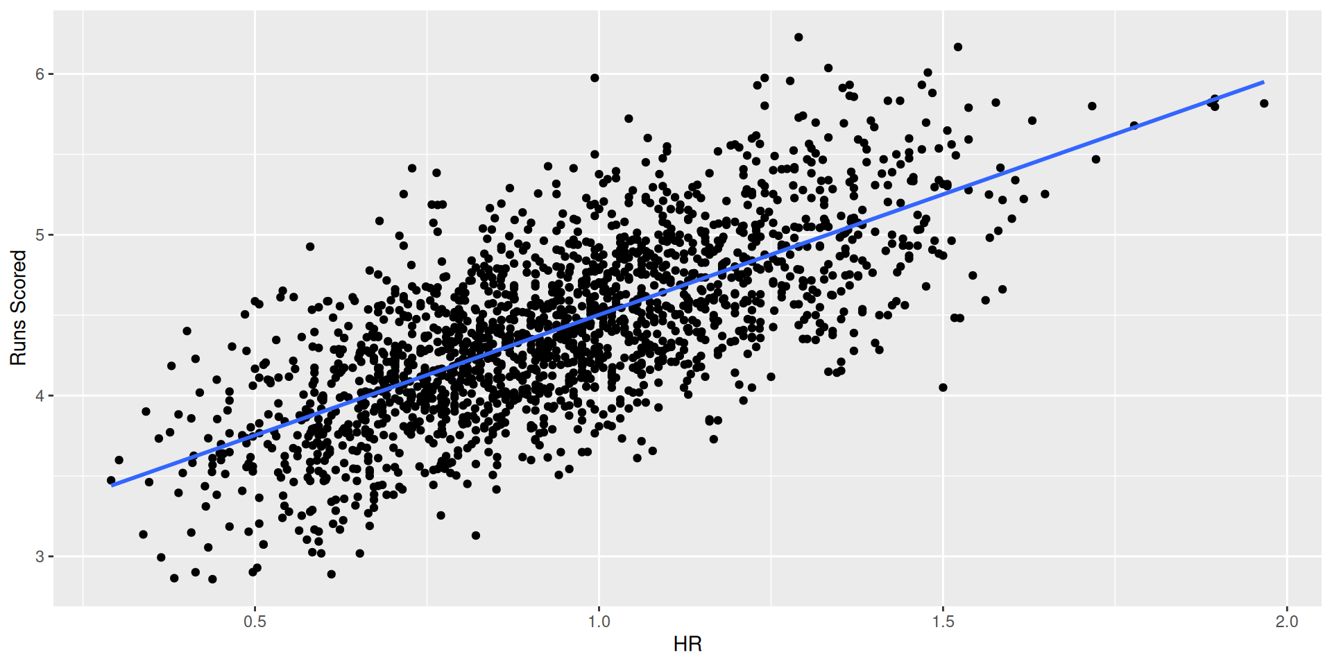
Regression model for home runs
Singles
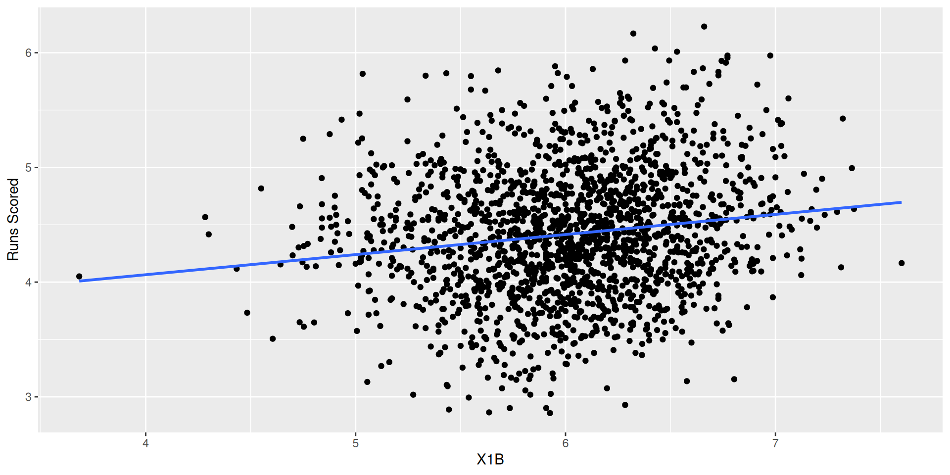
Regression model for singles
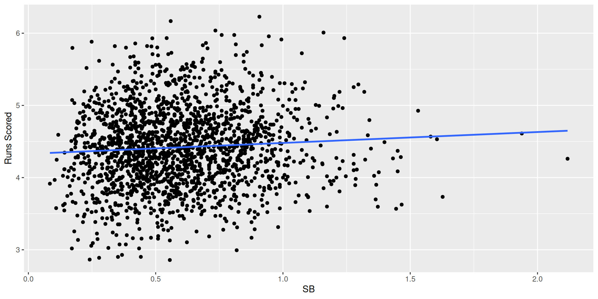
Stolen bases
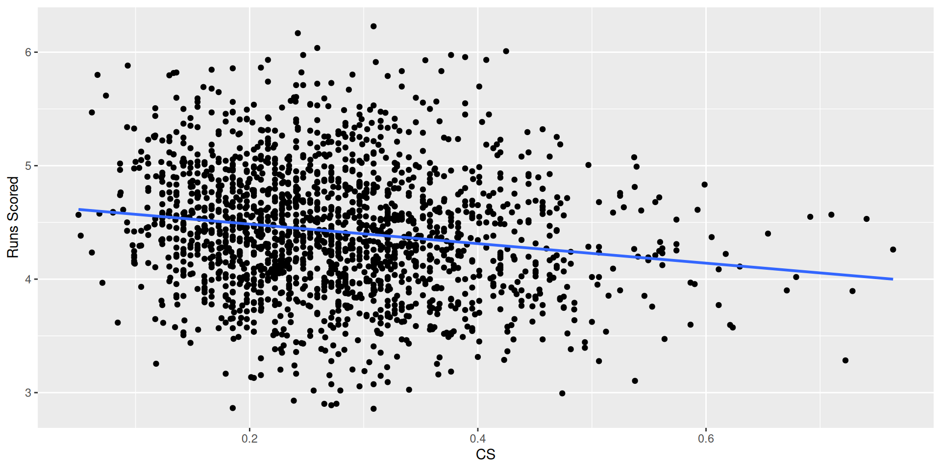
Caught stealings
Basic regression model
Call:
lm(formula = R ~ X1B + X2B + X3B + HR + WK + SB, data = filter(teams54rg,
    yearID < 2000))

Residuals:
     Min       1Q   Median       3Q      Max
-0.43719 -0.09737  0.00028  0.09707  0.47134

Coefficients:
            Estimate Std. Error t value Pr(>|t|)
(Intercept) -2.62043    0.08343 -31.410  < 2e-16 ***
X1B          0.51316    0.01261  40.703  < 2e-16 ***
X2B          0.61460    0.02399  25.623  < 2e-16 ***
X3B          1.29969    0.07083  18.351  < 2e-16 ***
HR           1.52896    0.02420  63.192  < 2e-16 ***
WK           0.34013    0.01074  31.659  < 2e-16 ***
SB           0.12645    0.01738   7.277 6.58e-13 ***
---
Signif. codes:  0 '***' 0.001 '**' 0.01 '*' 0.05 '.' 0.1 ' ' 1

Residual standard error: 0.1488 on 1071 degrees of freedom
Multiple R-squared:  0.9306,    Adjusted R-squared:  0.9302
F-statistic:  2394 on 6 and 1071 DF,  p-value: < 2.2e-16
Full regression model
Iterate over eras
# A tibble: 1 × 9
  `(Intercept)`   X1B   X2B   X3B    HR    WK    SB     CS   OUTS
          <dbl> <dbl> <dbl> <dbl> <dbl> <dbl> <dbl>  <dbl>  <dbl>
1 1.05 0.483 0.556 1.25 1.49 0.325 0.189 -0.267 -0.129# A tibble: 5 × 9
`(Intercept)` X1B X2B X3B HR WK SB CS OUTS
<dbl> <dbl> <dbl> <dbl> <dbl> <dbl> <dbl> <dbl> <dbl>
1 -0.245 0.541 0.491 0.845 1.63 0.374 0.299 0.0611 -0.0996
2 0.873 0.472 0.615 1.42 1.52 0.291 0.219 -0.363 -0.119
3 -0.320 0.505 0.679 1.02 1.46 0.336 0.208 -0.175 -0.0885
4 0.0815 0.503 0.770 1.09 1.50 0.312 0.168 -0.227 -0.110
5 1.60 0.365 0.777 1.63 1.40 0.298 0.211 -0.474 -0.130 Evaluating run estimators
Common run estimators
teams54 <- teams54 |>
mutate(
R = R/G,
BAVG = H / AB,
OBP = (H + WK) / (AB + WK + ifelse(is.na(SF), 0, SF)),
SLG = (X1B + 2*X2B + 3*X3B + 4*HR) / AB,
OPS = OBP + SLG,
LWTS = 0.46*X1B + 0.8*X2B + 1.02*X3B + 1.4*HR + 0.33*WK + 0.3*SB - 0.6*CS - 0.25*(OUTS),
XR = (0.5*X1B + 0.72*X2B + 1.04*X3B + 1.44*HR + 0.33*WK + 0.18*SB -0.32*CS - 0.098*OUTS) / G,
RC = OBP * SLG
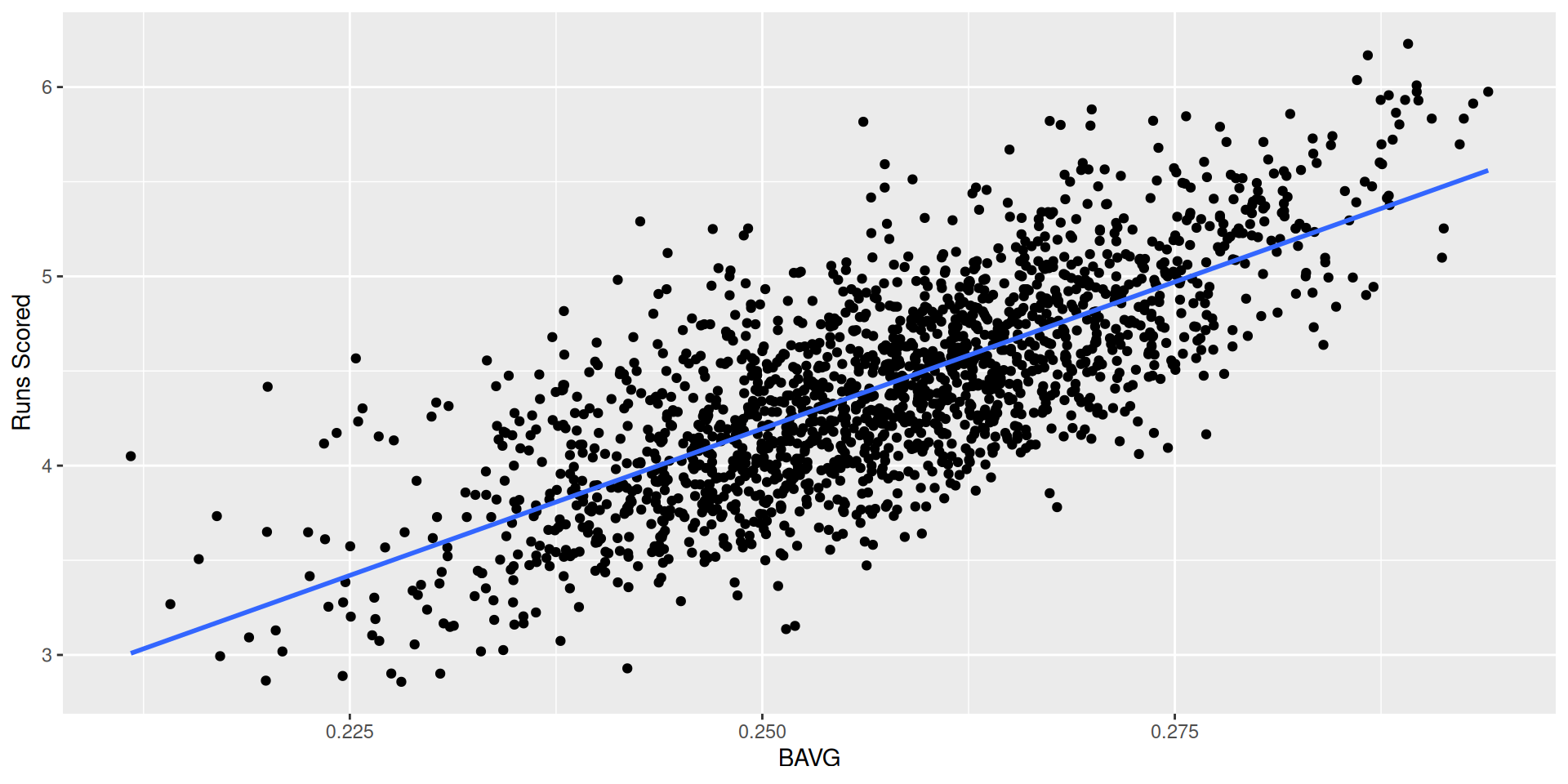
) Batting average
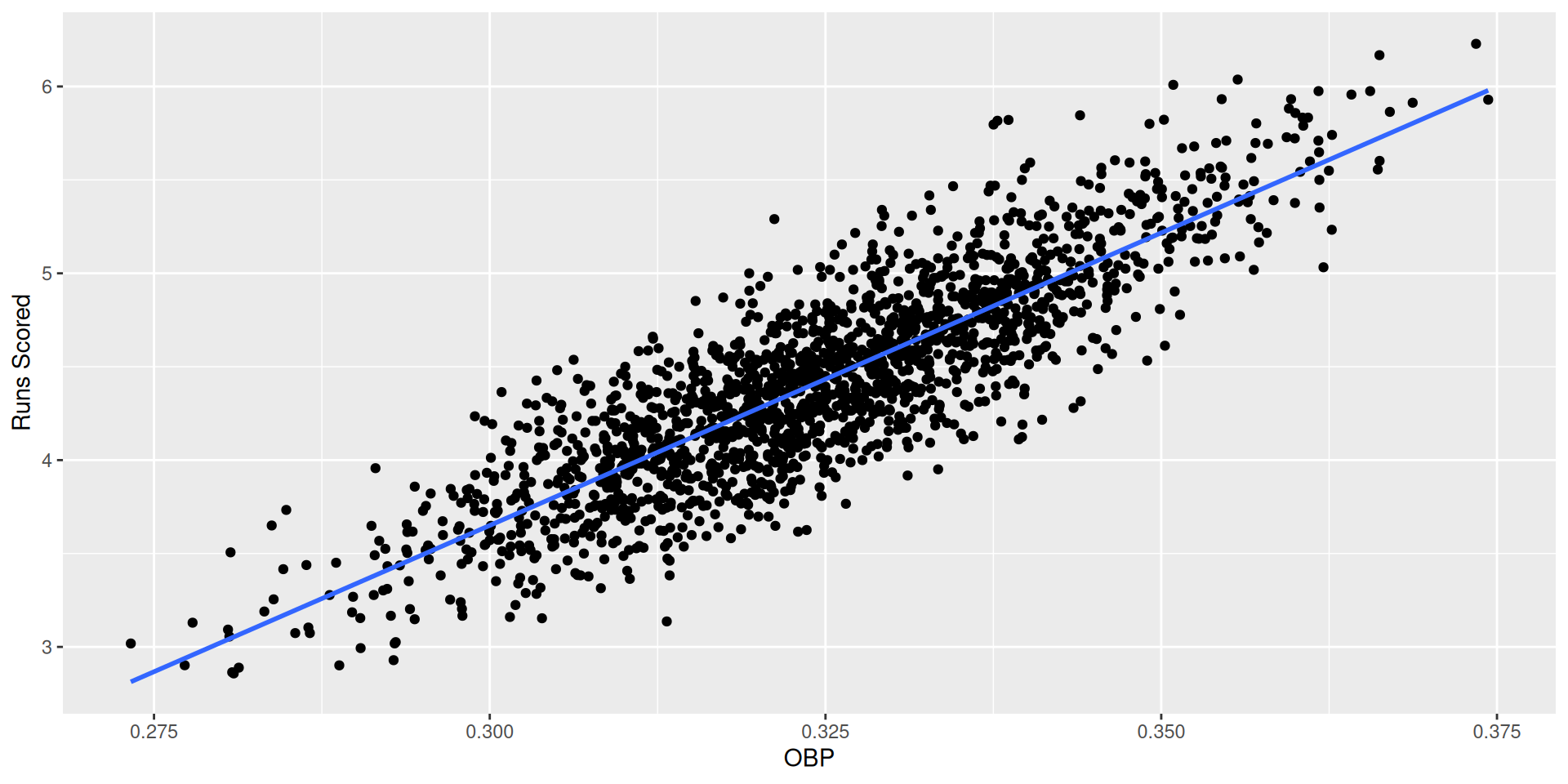
On-base percentage
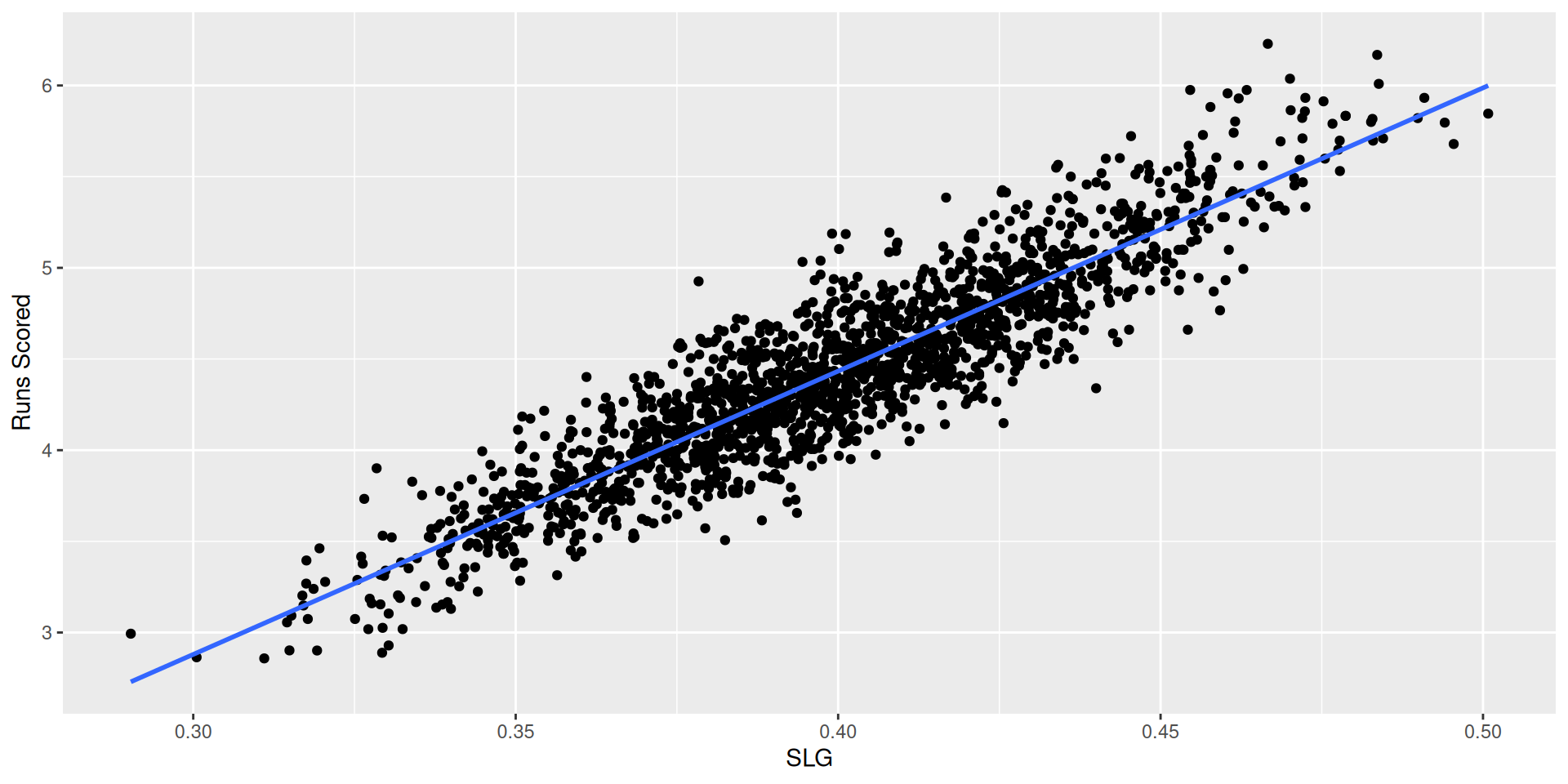
Slugging percentage
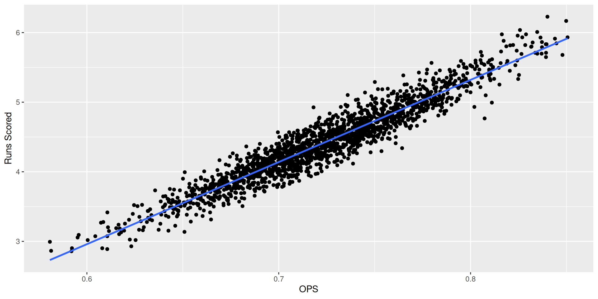
OPS
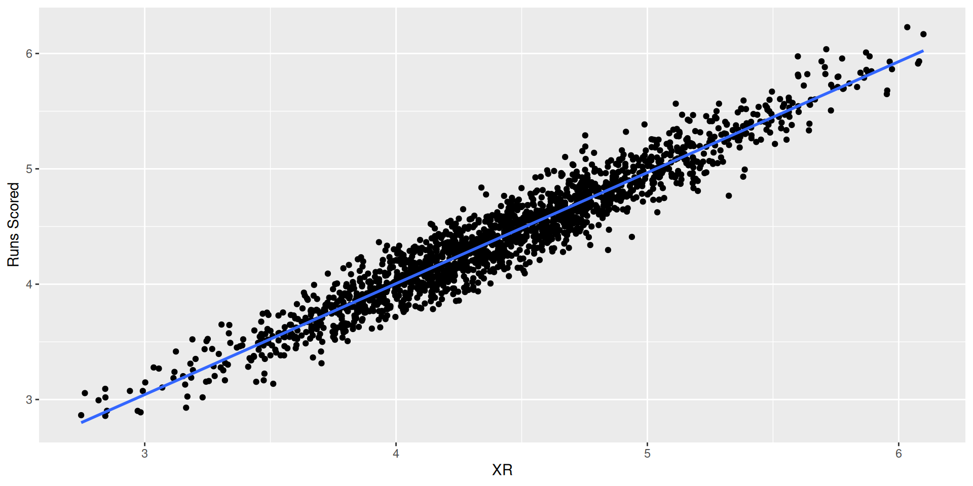
eXtrapolated Runs
Runs Created
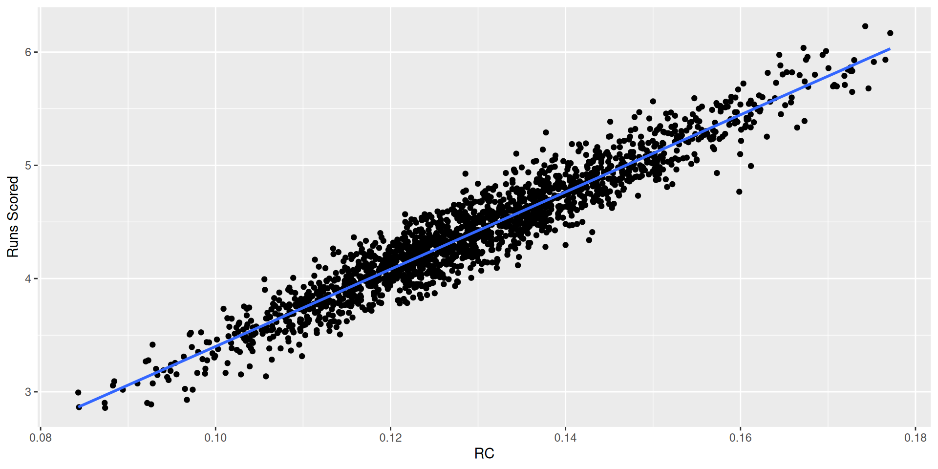
Correlation
             R      BAVG       OBP       SLG       OPS      LWTS        XR
R    1.0000000 0.7452374 0.8595853 0.9098903 0.9527274 0.9446182 0.9600107
BAVG 0.7452374 1.0000000 0.8414923 0.6821185 0.7812527 0.7709039 0.7790329
OBP  0.8595853 0.8414923 1.0000000 0.7242935 0.8657659 0.8839206 0.8904464
SLG  0.9098903 0.6821185 0.7242935 1.0000000 0.9721242 0.9355944 0.9483656
OPS  0.9527274 0.7812527 0.8657659 0.9721242 1.0000000 0.9796594 0.9911482
LWTS 0.9446182 0.7709039 0.8839206 0.9355944 0.9796594 1.0000000 0.9872646
XR   0.9600107 0.7790329 0.8904464 0.9483656 0.9911482 0.9872646 1.0000000
RC   0.9550842 0.7916800 0.8827493 0.9621475 0.9985340 0.9810157 0.9927272
            RC
R    0.9550842
BAVG 0.7916800
OBP  0.8827493
SLG  0.9621475
OPS  0.9985340
LWTS 0.9810157
XR   0.9927272
RC 1.0000000![]()
SDS 355