DIPS

SDS 355

Prof. Baumer

September 24, 2025

DIPS

The claim

There is little if any difference among major-league pitchers in their ability to prevent hits on balls hit in the field of play.

–Voros McCracken (2001)

The impact

A decade after Baseball Prospectus let McCracken spread the gospel in a story that popularized DIPS across the sport, it remains among the most seminal theories developed by sabermetrics, the nickname given to quantitative baseball study. It’s almost certainly the most revolutionary. Nothing before or since has so upended an entire line of thought and forced teams to assess a wide breadth of players in a different fashion.

– Jeff Passan (2011)

Who is Voros McCracken?

Voros McCracken is a student living in Chicago.

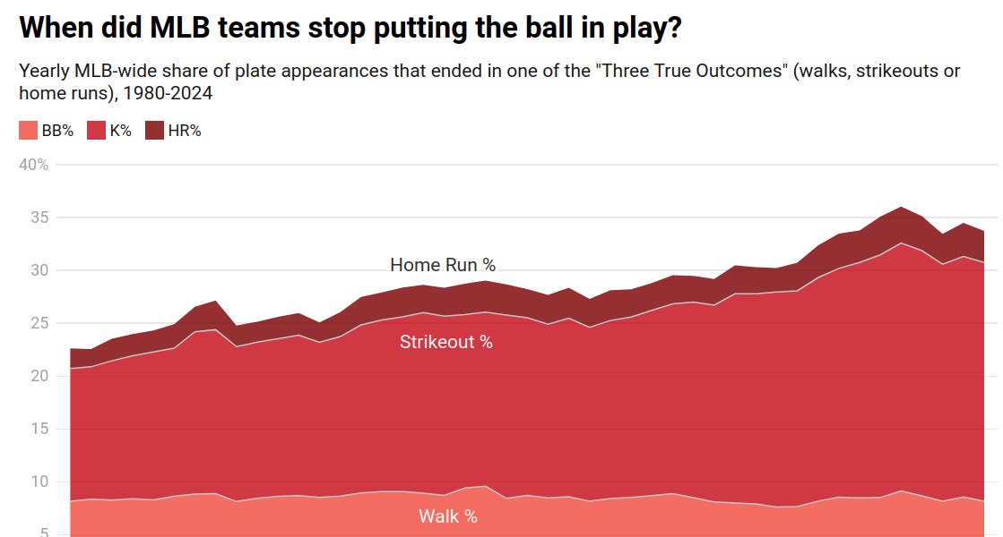
Outcomes of a plate appearance

• Balls in Play:
  • Hits
  • Outs
  • Errors

• Balls not in play (aka “Three true outcomes”):
  • Strikeouts
  • Walks / Hit by Pitch
  • Home Runs

Three True Outcomes

True outcomes over time

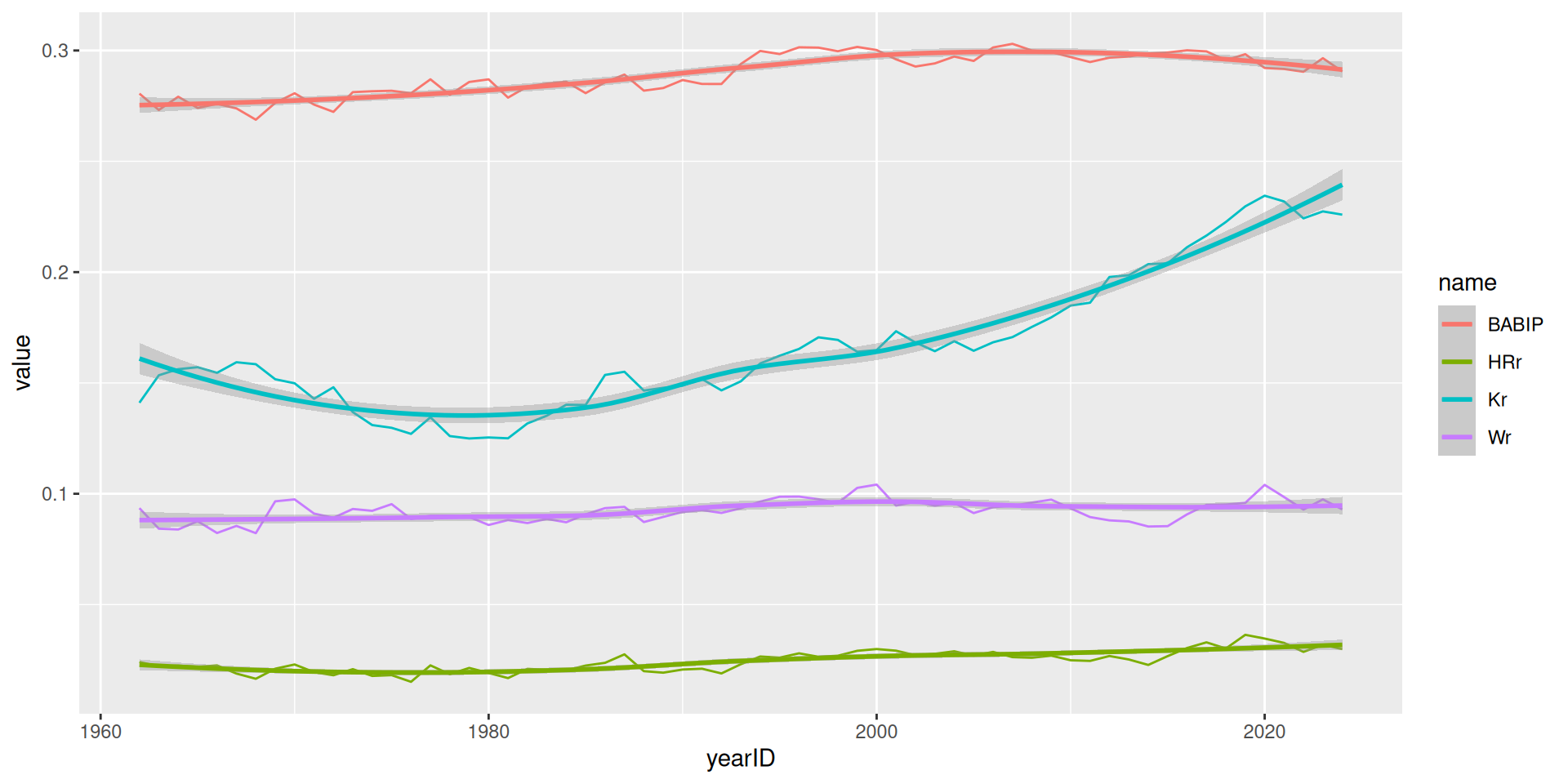
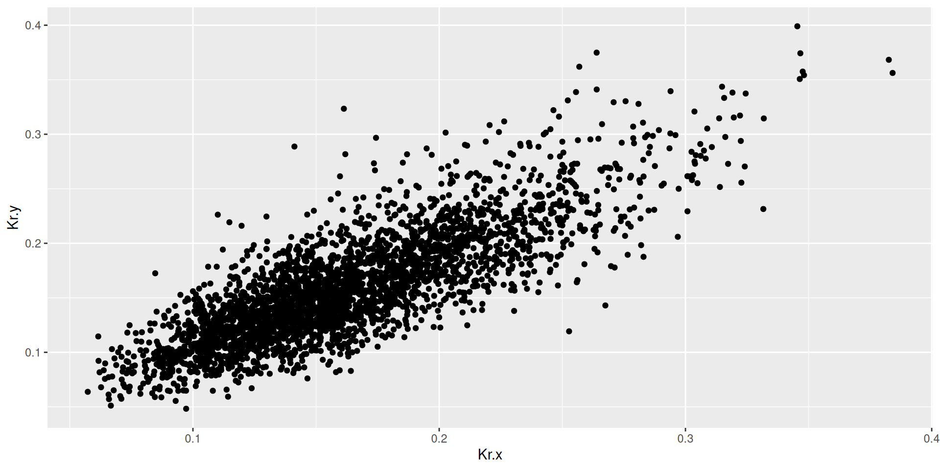
BABIP

Computing BABIP

library(tidyverse)
library(Lahman)

dips <- Batting |>
  filter(yearID >= 1962) |>
  group_by(yearID) |>
  summarize(
    TPA = sum(AB + BB + HBP + SF + SH),
    Kr = sum(SO) / TPA,
    Wr = sum(BB + HBP) / TPA,
    HRr = sum(HR) / TPA,
    BABIP = sum(H - HR) / sum(AB + SF - SO - HR) 
  )

True outcomes plot

dips |>
  pivot_longer(cols = Kr:BABIP) |>
  ggplot(aes(x = yearID, y = value, color = name)) +
  geom_line() + 
  geom_smooth()

Another claim

There is little correlation between what a pitcher does one year in the stat (BABIP) and what he will do the next.

The pitchers who are the best at preventing hits on balls in play one year are often the worst at it the next.

Fundamental question in sports analytics

• How much of performance is skill? How much is luck?

Pitcher-year pairs

dips_pitchers <- Pitching |>
  filter(yearID >= 1962) |>
  group_by(playerID, yearID) |>
  summarize(
    TPA = sum(BFP),
    Kr = sum(SO) / TPA,
    Wr = sum(BB + HBP) / TPA,
    HRr = sum(HR) / TPA,
    BABIP = sum(H - HR) / sum(BFP - BB - HBP - SO - HR),
  ) |>
  mutate(
    next_yearID = yearID + 1
  ) |>
  filter(TPA > 400)

dips_evens <- dips_pitchers |>
  filter(yearID %% 2 == 0)
dips_odds <- dips_pitchers |>
  filter(yearID %% 2 == 1)

dips_pairs <- dips_evens |>
  inner_join(dips_odds, by = join_by(playerID, next_yearID == yearID))

Paired data

dips_pairs |>
  head() |>
  select(contains("ID"), contains("BABIP"))

# A tibble: 6 × 6
# Groups:   playerID [3]
  playerID  yearID next_yearID next_yearID.y BABIP.x BABIP.y
  <chr>      <int>       <dbl>         <dbl>   <dbl>   <dbl>
1 aasedo01    1978        1979          1980   0.293   0.290
2 abbotgl01   1974        1975          1976   0.264   0.255
3 abbotgl01   1978        1979          1980   0.305   0.275
4 abbotgl01   1980        1981          1982   0.269   0.249
5 abbotji01   1990        1991          1992   0.316   0.277
6 abbotji01   1992        1993          1994   0.297   0.279

BABIP autocorrelation

dips_pairs |>
  ungroup() |>
  select(contains("BABIP")) |>
  cor()

          BABIP.x   BABIP.y
BABIP.x 1.0000000 0.2913783
BABIP.y 0.2913783 1.0000000

babip_plot <- ggplot(dips_pairs, aes(x = BABIP.x, y = BABIP.y)) +
  geom_point() +
  geom_label(
    data = filter(dips_pairs, playerID == "martipe02"),
    aes(label = yearID), color = "red"
  ) +
  scale_x_continuous("BABIP in some even year") +
  scale_y_continuous("BABIP in the next year")

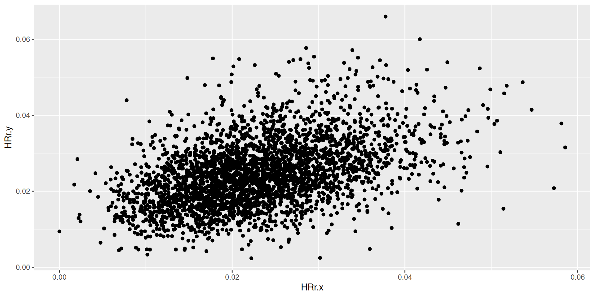
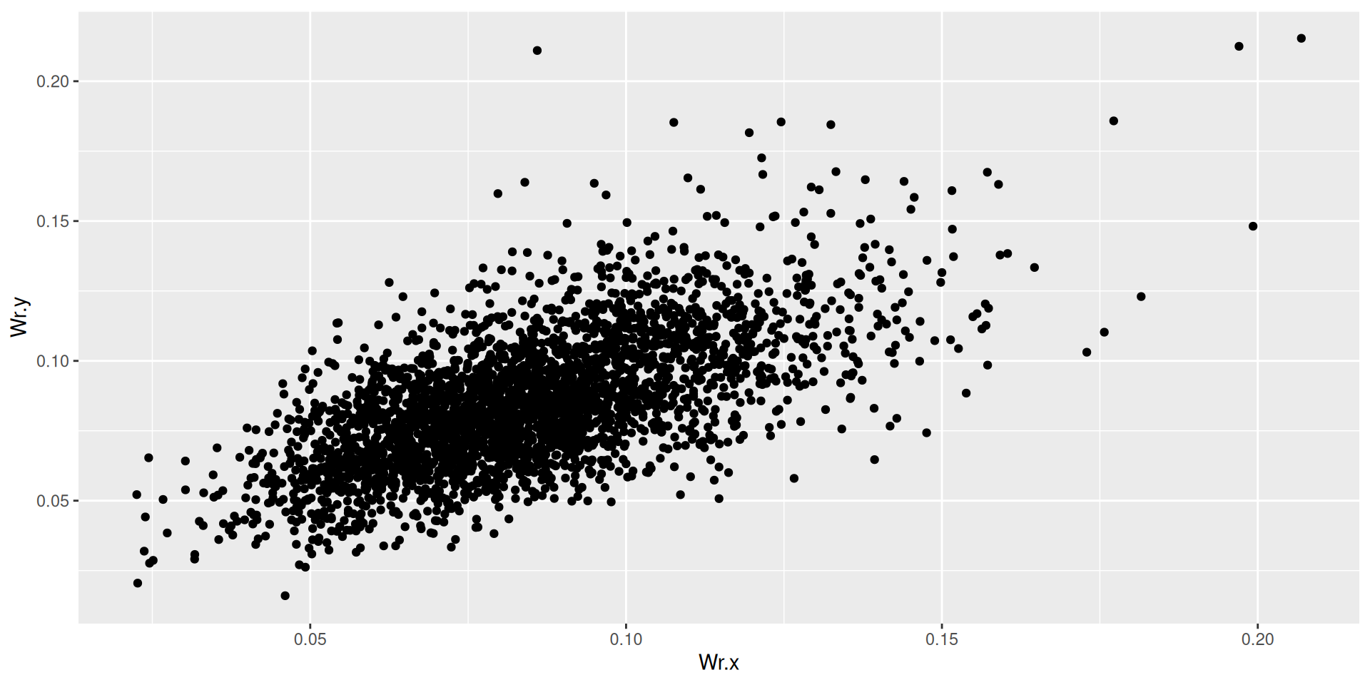
Visualizing BABIP autocorrelation

babip_plot

No cross-correlation

There is no significant cross-correlation. That is, a high number of home runs allowed doesn’t really mean anything in determining how many hits per balls in play the pitcher will allow.

Cross-correlations

dips_pairs |>
  ungroup() |>
  select(contains("r.x"), contains("BABIP")) |>
  cor() |>
  knitr::kable(digits = 2)

	Kr.x	Wr.x	HRr.x	BABIP.x	BABIP.y
Kr.x	1.00	0.10	0.09	0.06	0.04
Wr.x	0.10	1.00	-0.01	-0.02	-0.01
HRr.x	0.09	-0.01	1.00	0.08	0.12
BABIP.x	0.06	-0.02	0.08	1.00	0.29
BABIP.y	0.04	-0.01	0.12	0.29	1.00

Reliability

Home run rate

ggplot(dips_pairs, aes(x = HRr.x, y = HRr.y)) +
  geom_point()

Walk rate

ggplot(dips_pairs, aes(x = Wr.x, y = Wr.y)) +
  geom_point()

Strikeout rate

ggplot(dips_pairs, aes(x = Kr.x, y = Kr.y)) +
  geom_point()

Autocorrelations

dips_pairs |>
  ungroup() |>
  select(contains("r.")) |>
  cor() |>
  as_tibble(r, rownames = "stat") |>
  select(-contains(".x")) |>
  filter(str_detect(stat, ".x")) |>
  knitr::kable(digits = 2)

stat	Kr.y	Wr.y	HRr.y
Kr.x	0.82	0.08	0.13
Wr.x	0.13	0.64	-0.05
HRr.x	0.11	-0.06	0.46

FIP

Challenge

Calculate the year-to-year autocorrelation for FIP

What about batters?

stat	Kr.y	Wr.y	HRr.y	BABIP.y
Kr.x	0.88	0.22	0.48	0.12
Wr.x	0.21	0.77	0.34	-0.01
HRr.x	0.49	0.37	0.76	-0.05
BABIP.x	0.11	0.02	-0.01	0.46