Win Probability
SDS 355
Prof. Baumer
October 1, 2025
Win Probability
Super Bowl LI
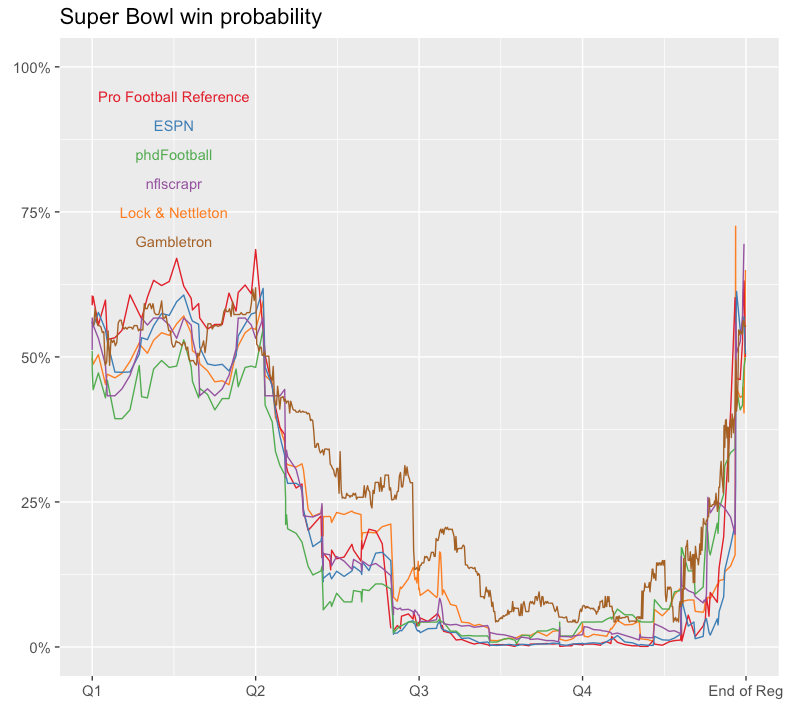
Pipping & Wyner (2025)
- A Paradox of Blown Leads: Rethinking Win Probability in Football
The most paradoxical and counterintuitive result of our study is that high win probabilities are not uncommon among teams that ultimately lose. In both simulated and real NFL games between evenly matched opponents, the losing team reached a win probability of at least 66–67% in half of all cases.
Pipping & Wyner (2025)

Computing Win Probability
Compute the score for each half inning
Half-innings
Determine the winners
Add the winners to the half-innings
# A tibble: 20,921 × 5
# Groups:   game_id [2,428]
   game_id      inn_ct home_lead final_score is_home_win
   <chr>         <int>     <int>       <int> <lgl>
 1 ANA201604040      1        -1          -9 FALSE
 2 ANA201604040      2        -1          -9 FALSE
 3 ANA201604040      3        -1          -9 FALSE
 4 ANA201604040      4        -3          -9 FALSE
 5 ANA201604040      5        -3          -9 FALSE
 6 ANA201604040      6        -5          -9 FALSE
 7 ANA201604040      7        -6          -9 FALSE
 8 ANA201604040      8        -6          -9 FALSE
 9 ANA201604040      9        -9          -9 FALSE
10 ANA201604050      1         0          -5 FALSE
# ℹ 20,911 more rows
Fit the logistic regression models for each inning
# A tibble: 10 × 2
   `(Intercept)` home_lead
           <dbl>     <dbl>
 1       0.0330      0.515
 2       0.0152      0.488
 3      -0.0111      0.502
 4      -0.00177     0.586
 5      -0.0225      0.646
 6      -0.0369      0.811
 7      -0.0739      1.04
 8      -0.142       1.61
 9       0.593      20.2
10       0.560      18.3
Make a prediction
- For a 2-run lead in the 4th inning:
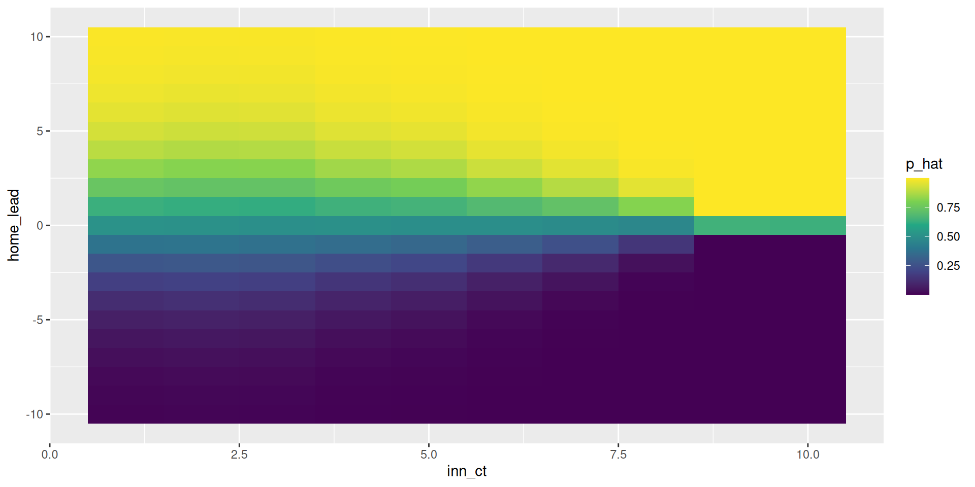
Flesh out the grid of expected win probabilities
View the grid
| -10 | -9 | -8 | -7 | -6 | -5 | -4 | -3 | -2 | -1 | 0 | 1 | 2 | 3 | 4 | 5 | 6 | 7 | 8 | 9 | 10 | inn_ct |
|---|---|---|---|---|---|---|---|---|---|---|---|---|---|---|---|---|---|---|---|---|---|
| 0.01 | 0.01 | 0.02 | 0.03 | 0.04 | 0.07 | 0.12 | 0.18 | 0.27 | 0.38 | 0.51 | 0.63 | 0.74 | 0.83 | 0.89 | 0.93 | 0.96 | 0.97 | 0.98 | 0.99 | 0.99 | 1 |
| 0.01 | 0.01 | 0.02 | 0.03 | 0.05 | 0.08 | 0.13 | 0.19 | 0.28 | 0.38 | 0.50 | 0.62 | 0.73 | 0.81 | 0.88 | 0.92 | 0.95 | 0.97 | 0.98 | 0.99 | 0.99 | 2 |
| 0.01 | 0.01 | 0.02 | 0.03 | 0.05 | 0.07 | 0.12 | 0.18 | 0.27 | 0.37 | 0.50 | 0.62 | 0.73 | 0.82 | 0.88 | 0.92 | 0.95 | 0.97 | 0.98 | 0.99 | 0.99 | 3 |
| 0.00 | 0.01 | 0.01 | 0.02 | 0.03 | 0.05 | 0.09 | 0.15 | 0.24 | 0.36 | 0.50 | 0.64 | 0.76 | 0.85 | 0.91 | 0.95 | 0.97 | 0.98 | 0.99 | 0.99 | 1.00 | 4 |
| 0.00 | 0.00 | 0.01 | 0.01 | 0.02 | 0.04 | 0.07 | 0.12 | 0.21 | 0.34 | 0.49 | 0.65 | 0.78 | 0.87 | 0.93 | 0.96 | 0.98 | 0.99 | 0.99 | 1.00 | 1.00 | 5 |
| 0.00 | 0.00 | 0.00 | 0.00 | 0.01 | 0.02 | 0.04 | 0.08 | 0.16 | 0.30 | 0.49 | 0.68 | 0.83 | 0.92 | 0.96 | 0.98 | 0.99 | 1.00 | 1.00 | 1.00 | 1.00 | 6 |
| 0.00 | 0.00 | 0.00 | 0.00 | 0.00 | 0.01 | 0.01 | 0.04 | 0.10 | 0.25 | 0.48 | 0.72 | 0.88 | 0.95 | 0.98 | 0.99 | 1.00 | 1.00 | 1.00 | 1.00 | 1.00 | 7 |
| 0.00 | 0.00 | 0.00 | 0.00 | 0.00 | 0.00 | 0.00 | 0.01 | 0.03 | 0.15 | 0.46 | 0.81 | 0.96 | 0.99 | 1.00 | 1.00 | 1.00 | 1.00 | 1.00 | 1.00 | 1.00 | 8 |
| 0.00 | 0.00 | 0.00 | 0.00 | 0.00 | 0.00 | 0.00 | 0.00 | 0.00 | 0.00 | 0.64 | 1.00 | 1.00 | 1.00 | 1.00 | 1.00 | 1.00 | 1.00 | 1.00 | 1.00 | 1.00 | 9 |
| 0.00 | 0.00 | 0.00 | 0.00 | 0.00 | 0.00 | 0.00 | 0.00 | 0.00 | 0.00 | 0.64 | 1.00 | 1.00 | 1.00 | 1.00 | 1.00 | 1.00 | 1.00 | 1.00 | 1.00 | 1.00 | 10 |
Visualize win probabilities
Write function to compute fitted values
[1] 0.2695287 0.3838537 0.4972250 0.6420287Bring in the Expected Run Matrix
erm2016 <- read_rds(here::here("data/erm2016.rda"))

wpa <- retro2016 |>
  filter(game_id == "ANA201604070") |>
  retrosheet_add_states() |>
  mutate(home_lead = home_score_ct - away_score_ct) |>
  left_join(erm2016, by = join_by(bases, outs_ct)) |>
  mutate(
    exp_home_lead = home_lead + ifelse(bat_home_id == 1, exp_run_value, -exp_run_value),
    p_hat = predict_wp(inn_ct, home_lead),
    p_hat_exp = predict_wp(inn_ct, exp_home_lead)
  )
Spot check
# A tibble: 76 × 11
   event_id bat_home_id inn_ct bases outs_ct bat_id   home_lead exp_run_value
      <int>       <int>  <int> <chr>   <int> <chr>        <int>         <dbl>
 1        1           0      1 000         0 deshd002         0         0.498
 2        2           0      1 100         0 choos001         0         0.858
 3        3           0      1 110         0 belta001         0         1.44
 4        4           0      1 110         1 fielp001         0         0.921
 5        5           0      1 011         1 fielp001         0         1.36
 6        6           0      1 010         2 desmi001        -1         0.312
 7        7           1      1 000         0 escoy001        -1         0.498
 8        8           1      1 000         1 gentc001        -1         0.268
 9        9           1      1 000         2 troum001        -1         0.106
10       10           1      1 100         2 pujoa001        -1         0.220
# ℹ 66 more rows
# ℹ 3 more variables: exp_home_lead <dbl>, p_hat <dbl>, p_hat_exp <dbl>
Win probability plot
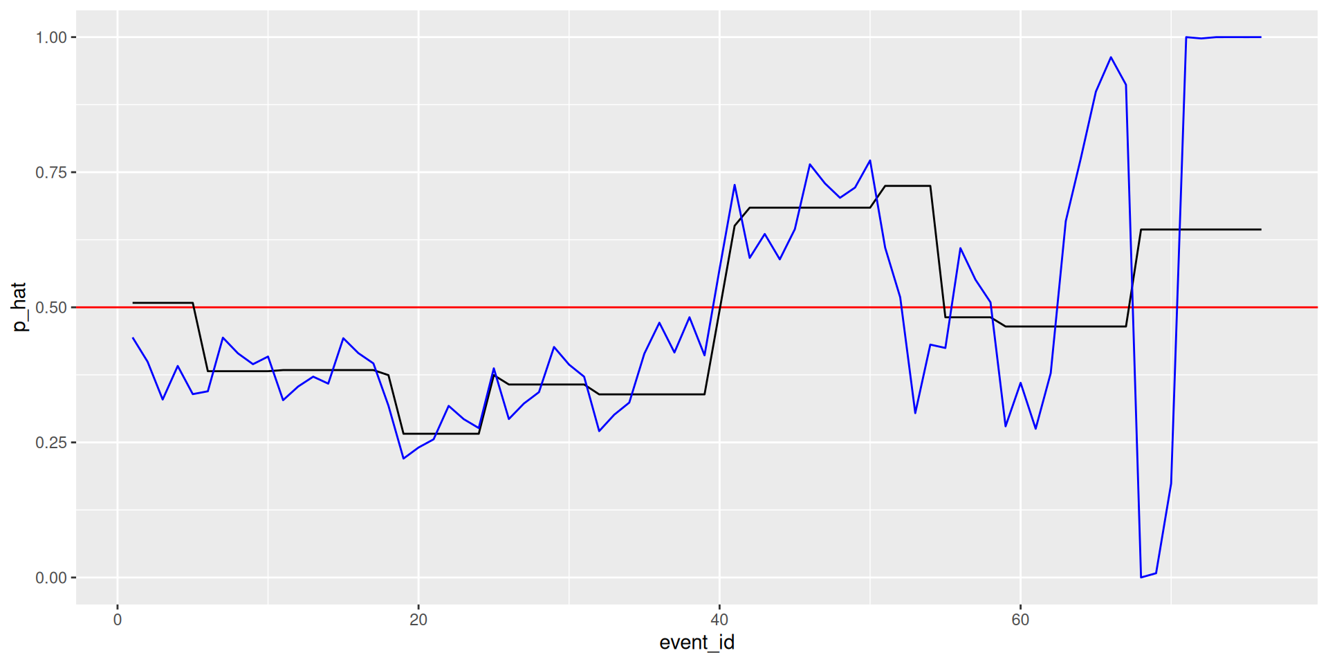
What happened?
Win probability added
wpa |>
  mutate(
    next_p_hat = lead(p_hat, default = 1),
    next_p_hat_exp = lead(p_hat_exp, default = 1)
  ) |>
#  select(event_id, inn_ct, bases, outs_ct, bat_id, home_lead, exp_run_value, exp_home_lead, p_hat, next_p_hat) |> view()
  group_by(bat_id) |>
  summarize(
    wpa = sum(next_p_hat - p_hat, na.rm = TRUE),
    wpa_exp = sum(next_p_hat_exp - p_hat_exp, na.rm = TRUE)
  ) |>
  arrange(desc(wpa))
# A tibble: 20 × 3
bat_id wpa wpa_exp
<chr> <dbl> <dbl>
1 pujoa001 0.358 -0.0150
2 escoy001 0.264 0.200
3 simma001 0.170 -0.995
4 gentc001 0.122 -0.188
5 sotog001 0.0403 -0.121
6 troum001 0.0334 -0.0374
7 belta001 0 0.283
8 calhk001 0 0.00623
9 choij001 0 -0.00241
10 choos001 0 -0.187
11 deshd002 0 0.100
12 desmi001 0 0.0363
13 giavj001 0 -0.143
14 morem001 0 0.0605
15 odorr001 0 1.00
16 perec003 0 -0.00000835
17 cronc002 -0.0183 -0.0912
18 chirr001 -0.108 0.261
19 fielp001 -0.126 0.383
20 andre001 -0.243 0.00329 ![]()
SDS 355