library(rvest)
scrape_standings <- function(year = 2025) {
url <- paste0("https://www.basketball-reference.com/leagues/NBA_", year, ".html")
x <- url |>
read_html() |>
html_table()
x[1:2] |>
map(janitor::clean_names) |>
map(rename_with, ~str_remove(.x, "eastern_|western_"), contains("conference")) |>
list_rbind() |>
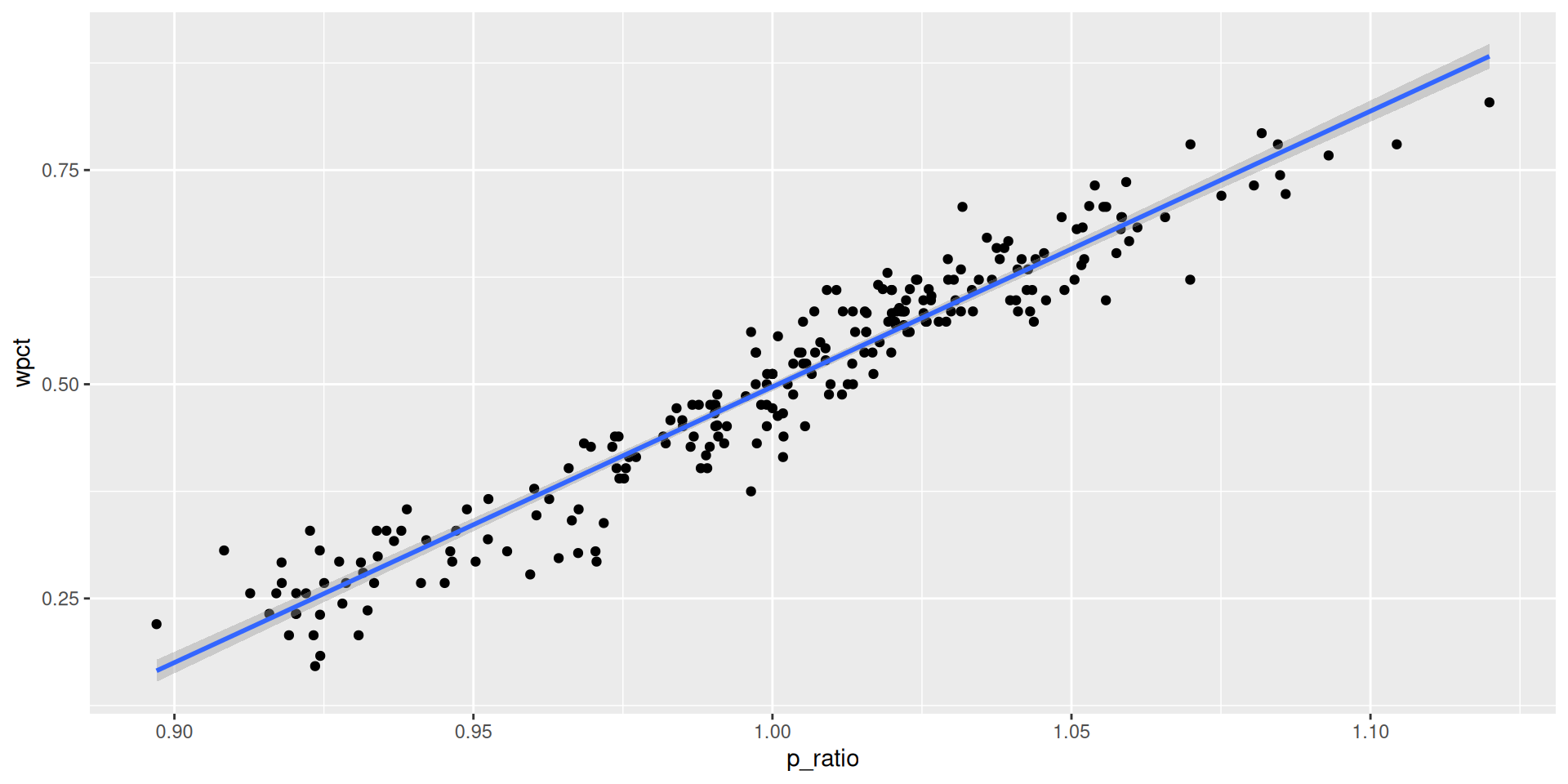
mutate(
p_ratio = ps_g / pa_g,
wpct = w_l_percent,
logWratio = log(w / l),
logPratio = log(ps_g / pa_g)
)
}Four Factors
SDS 355
October 5, 2025
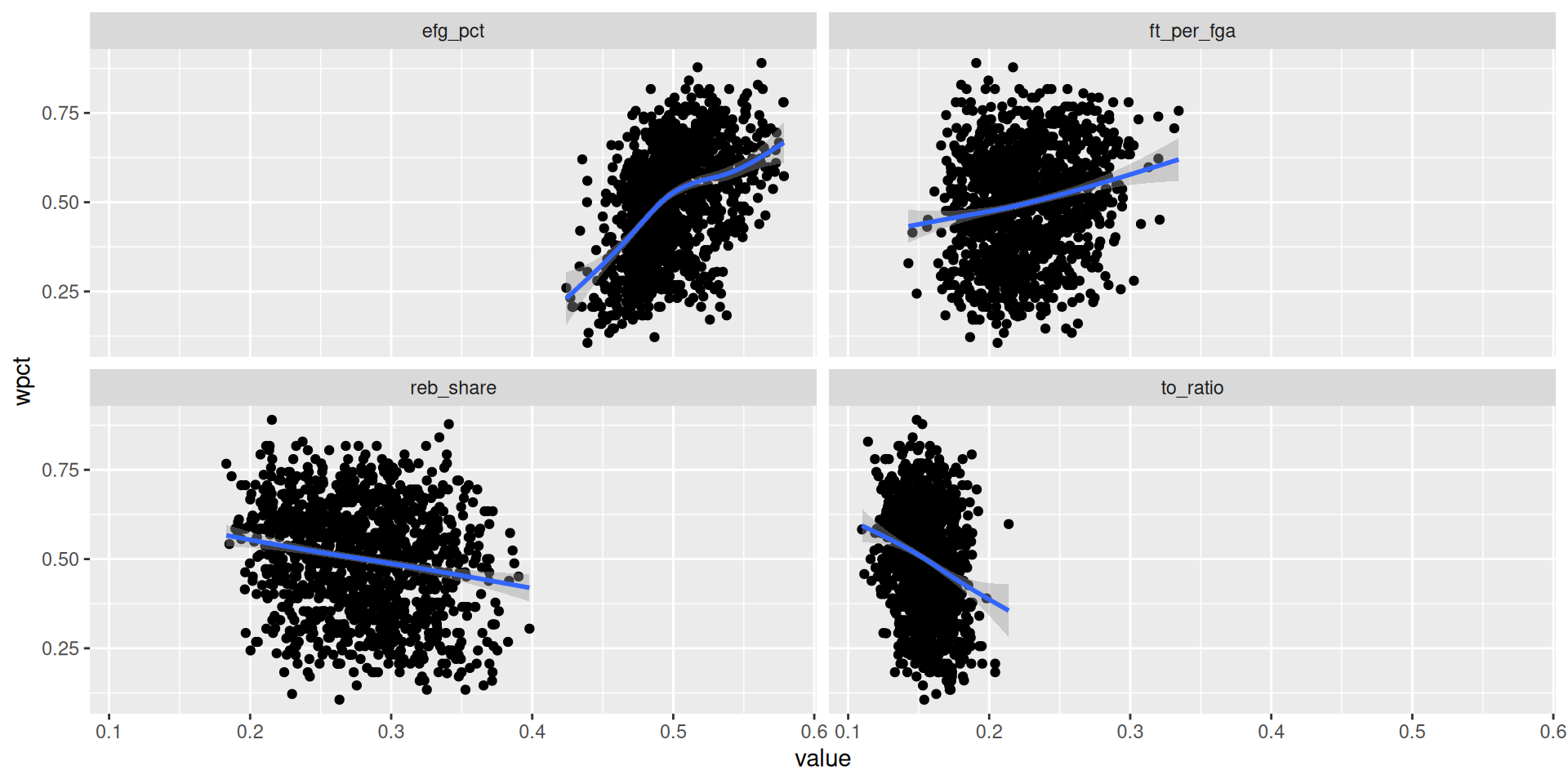
Visualize the relationship
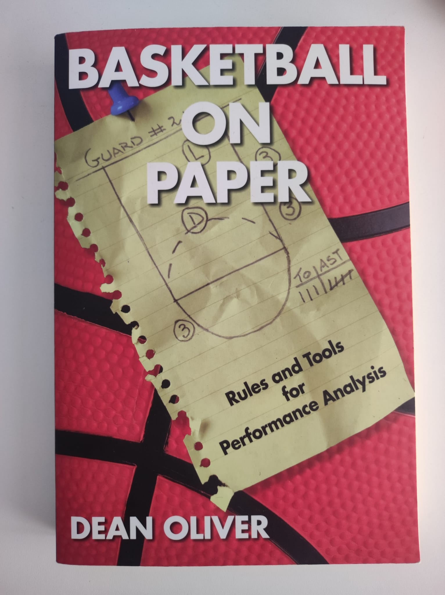
Dean Oliver, Basketball on Paper

Effective field goal percentage
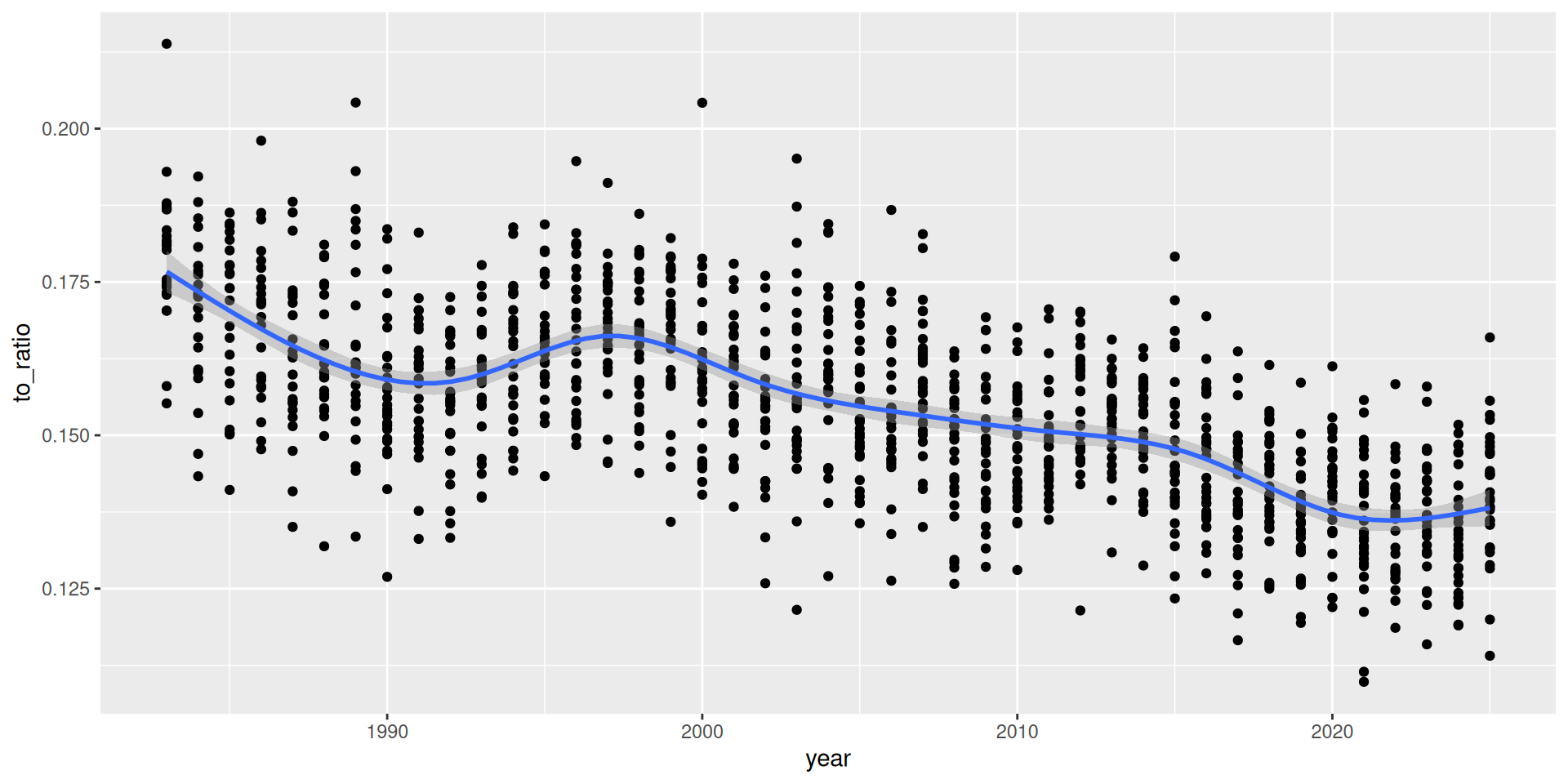
Turnover ratio
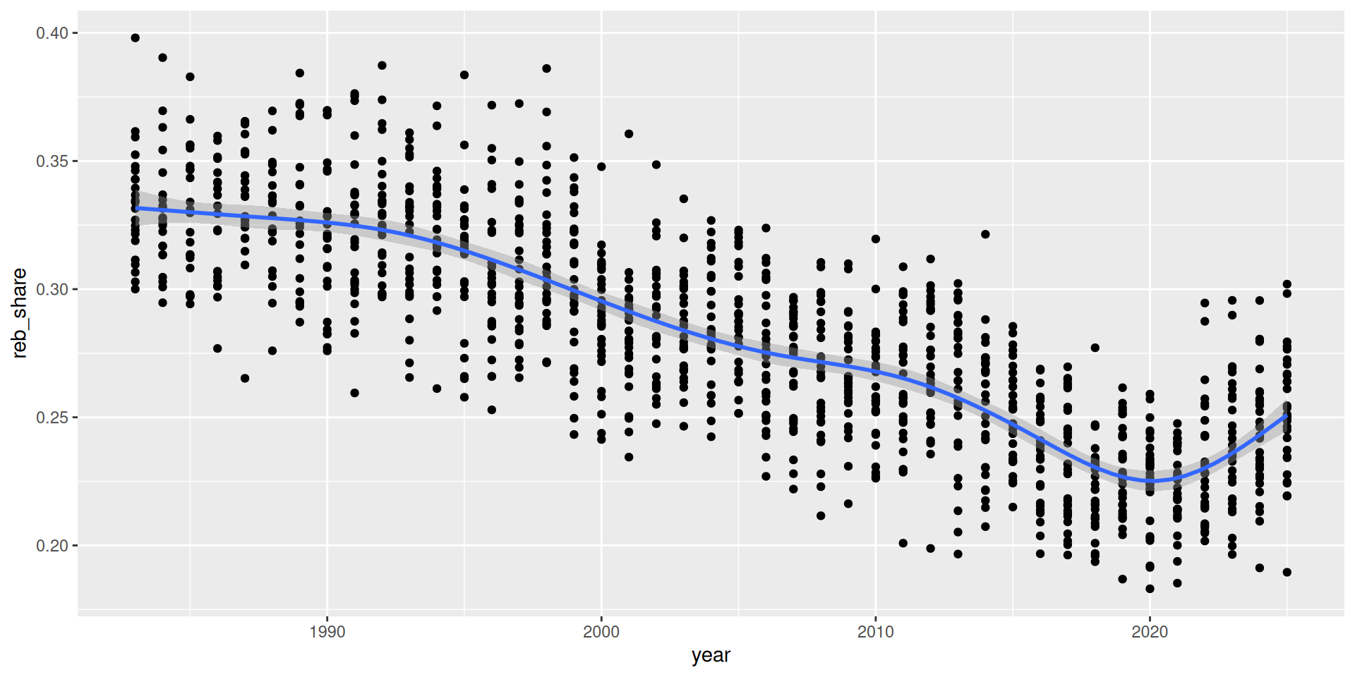
Offensive rebound percentage
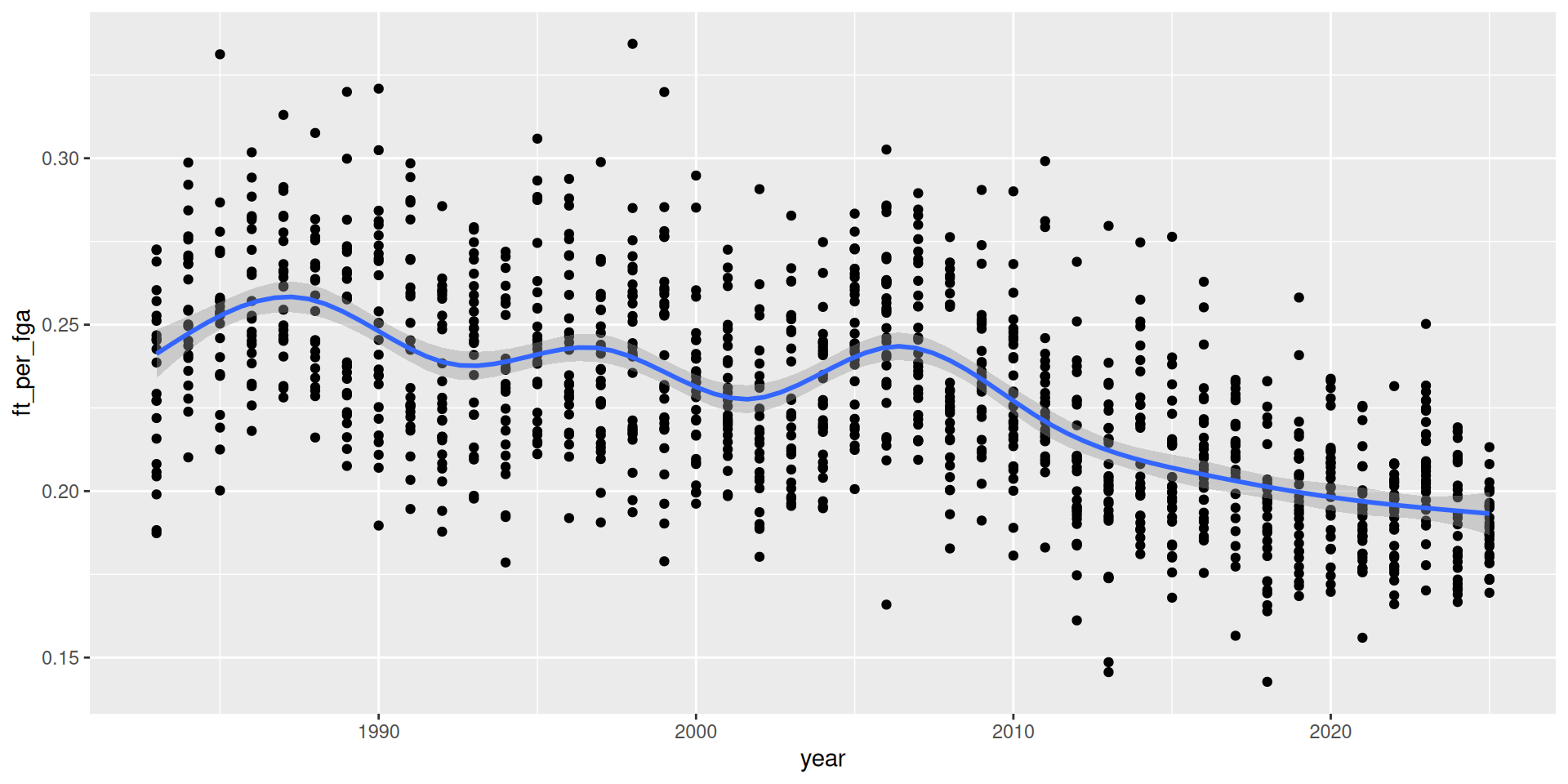
Free throw conversion rate
The Four Factors, visualized
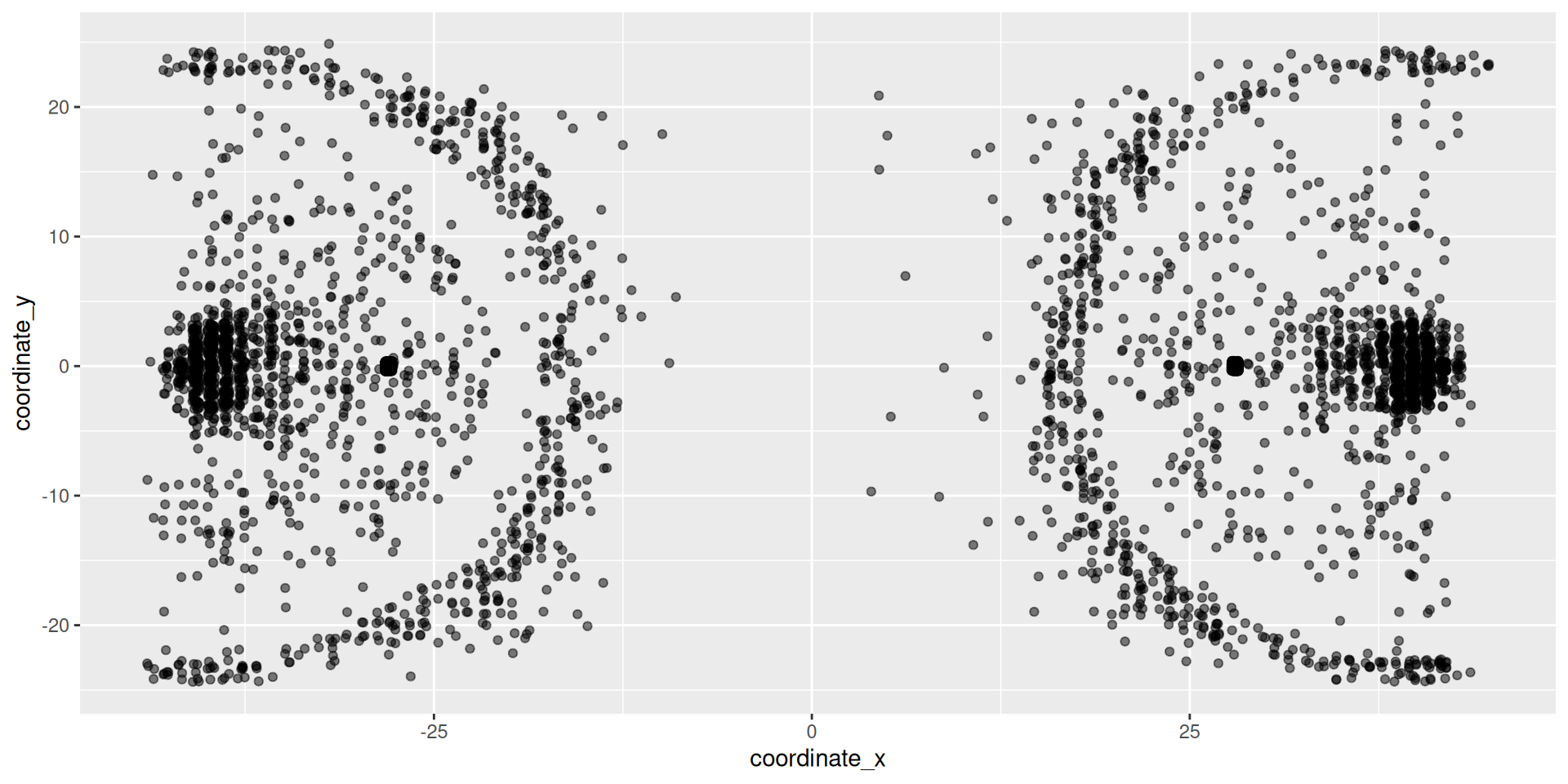
Shot chart
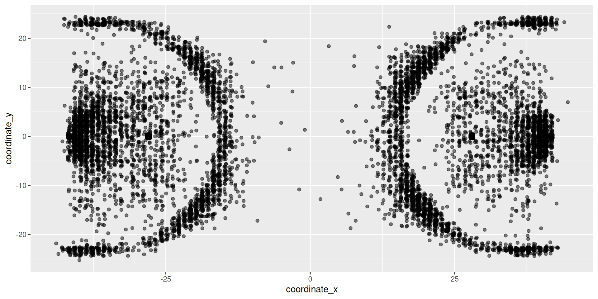
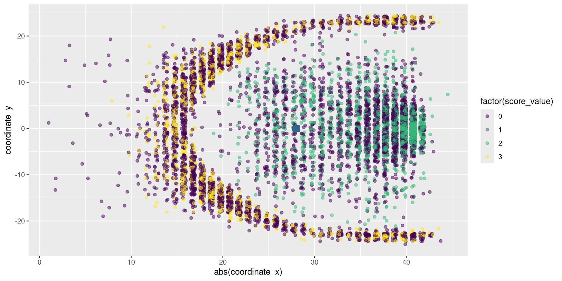
Halfcourt
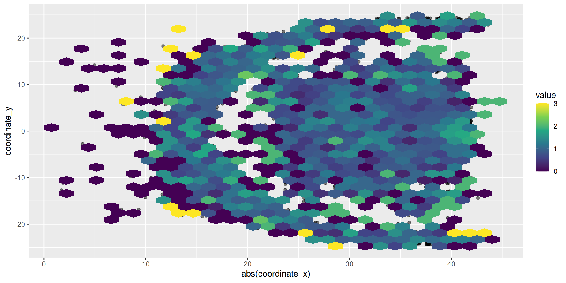
Hex bin plot
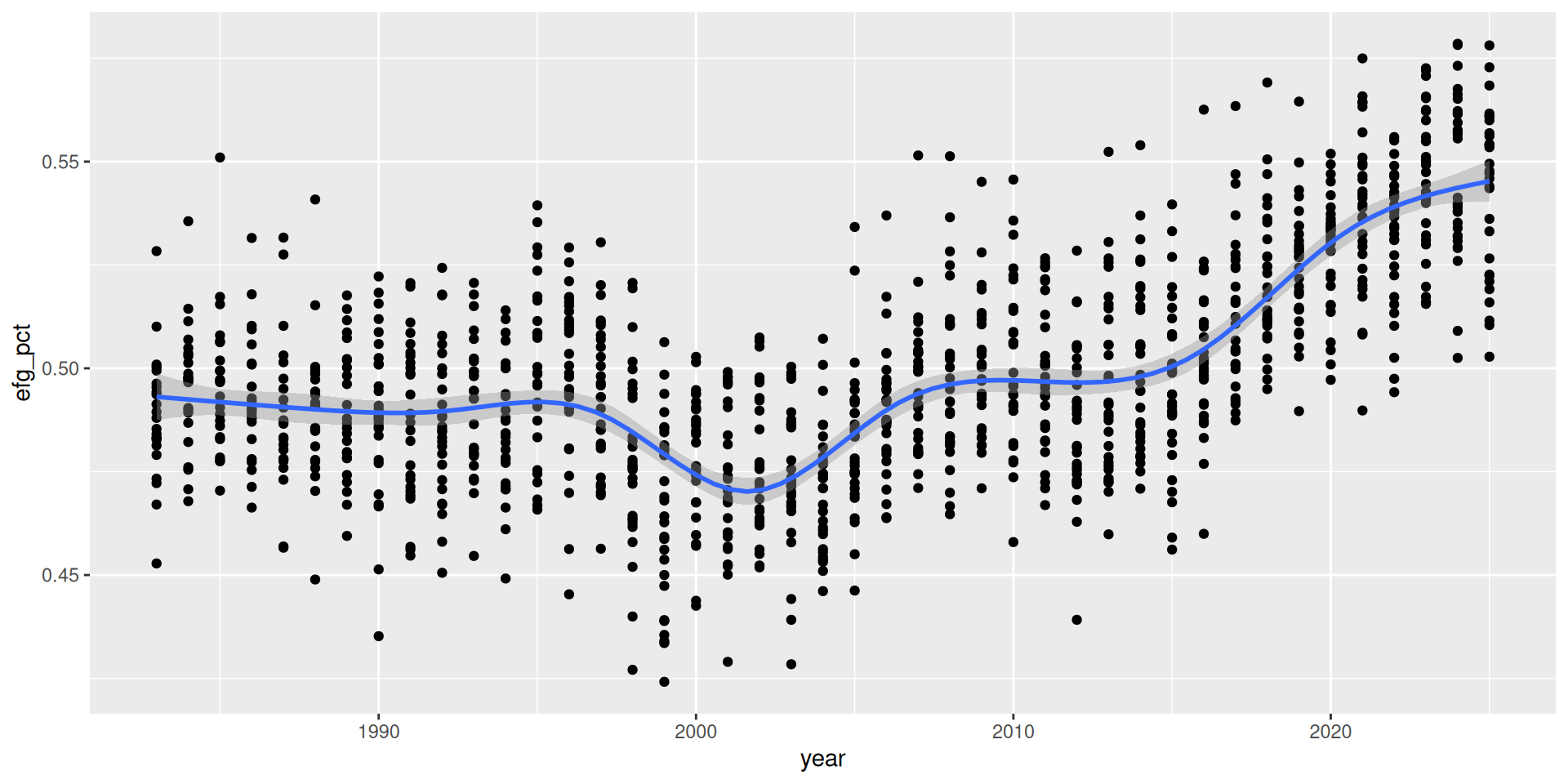
The game has changed

Add the court lines with sportyR
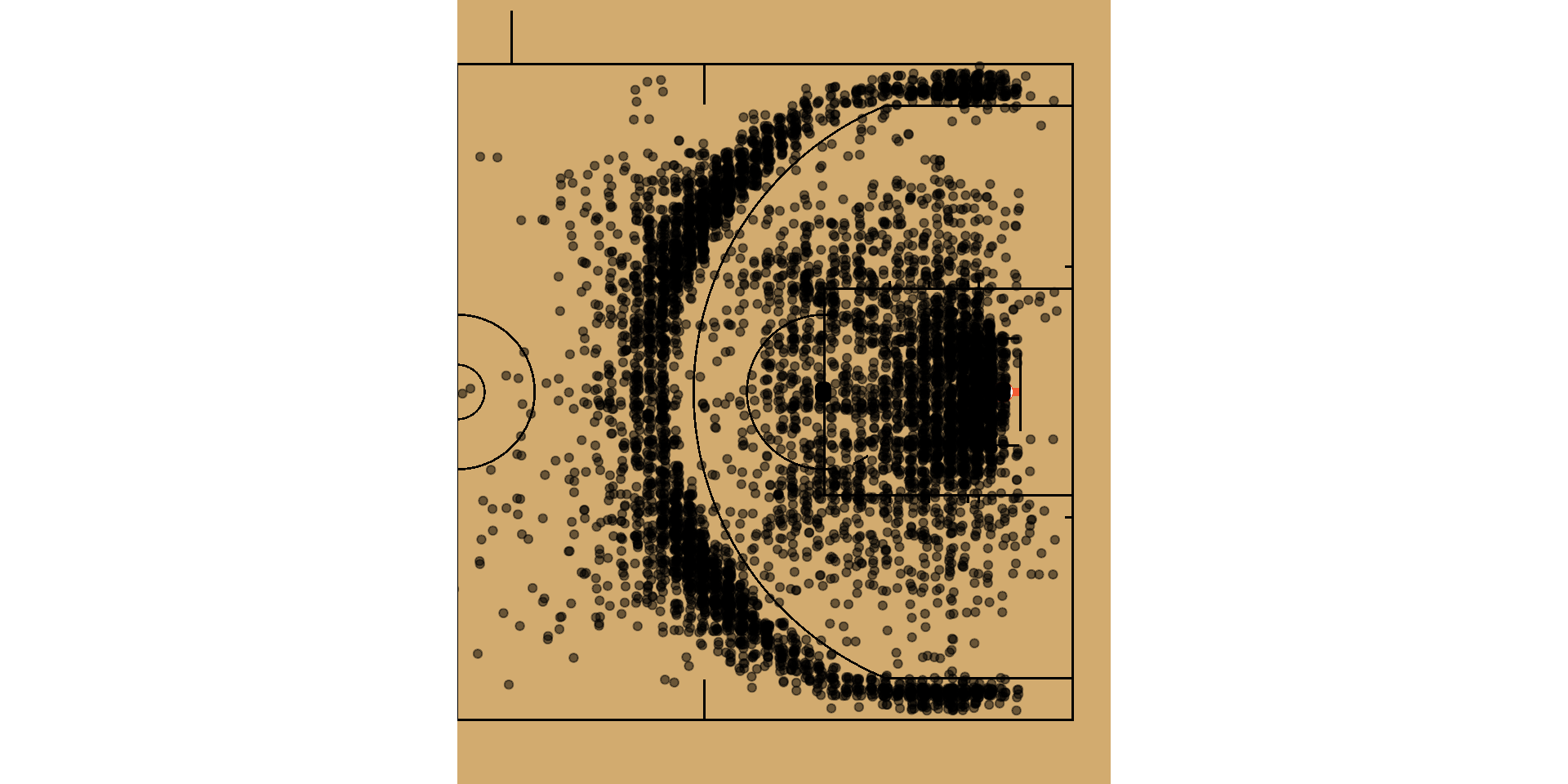
wehoop
![]()
WNBA shot chart