tidychangepoint

a unified framework for analyzing changepoint detection in univariate time series

Benjamin S. Baumer, Smith College

Universitat Politècnica de Catalunya

2025-06-27

Changepoint Detection

Changepoint Detection Problem (CDP)

• Given a time series \(y = \{y_1, \ldots, y_n \} \in \mathbb{R}^n\)
• A set of indices \(\tau = \{ \tau_1, \ldots, \tau_m \} \in [1,n]^m\) is a changepoint set
• Find the changepoint set that minimizes some penalized objective function (that acts on \(\tau\))

A change point is an abrupt change in the time line of observation of some phenomenon. Studying these points provides insight into patterns of behavior and transitions between cycles. Change points divide the time series into segments or intervals that are not necessarily independent or identically distributed. Although these concepts have been present in time series models for a long time, methods have recently been developed that avoid assuming a specific distribution for the random mechanism that generates the observations over time. Both classical and emergent models have demonstrated effectiveness in fitting time series and in identifying how many change points exist and where they are located.

Why is CDP hard?

• Search space is exponentially large (\(2^n\) possible changepoint sets)
• Many different ways to model the time series (parametrically)
• Many different penalty functions (e.g., BIC, MDL, etc.)
• No real “ground truth”

Ex. 1: History of the designated hitter

Ex. 1: Controversy

Ex. 1: Difference in HR rate

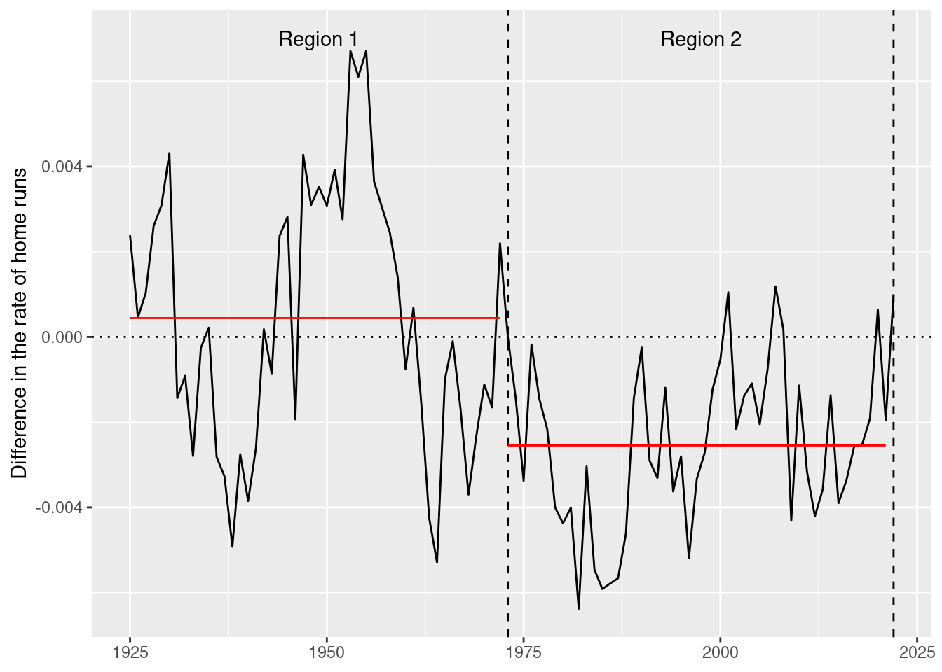
• True changepoint is known (1973)
• Can we find it?

Difference in the rate of home runs per plate appearance between the American and National Leagues in Major League Baseball, 1925–2022. The designated hitter rule was adopted in 1973 by the American League, but not until 2022 by the National League. Note how, during the period from 1973 to 2022 when only the American League employed a designated hitter, the difference in home run rate was nearly always negative.

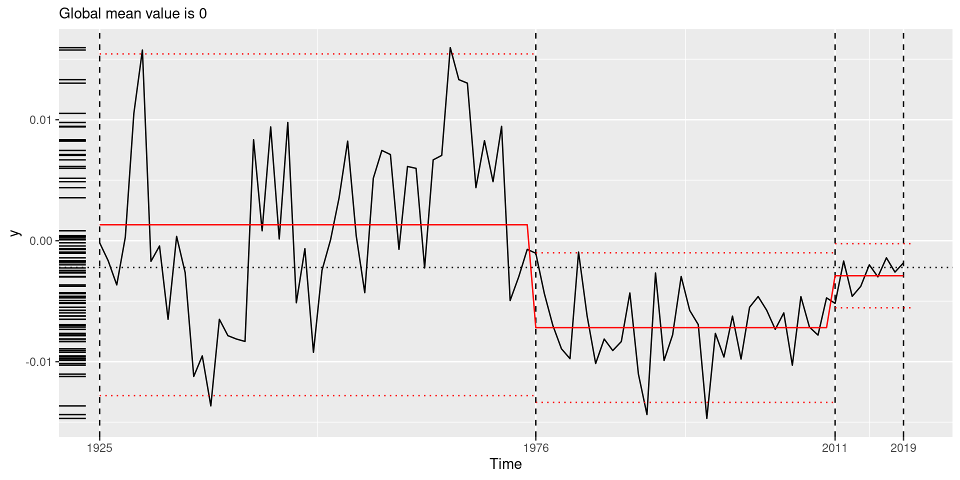
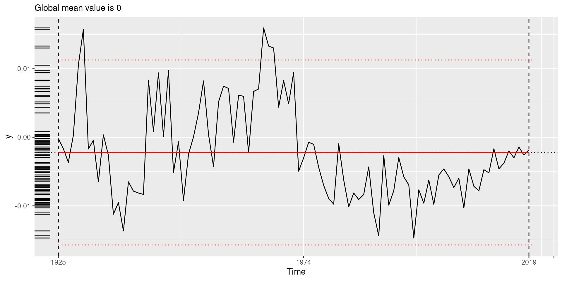
Ex. 1B: Expert-defined eras

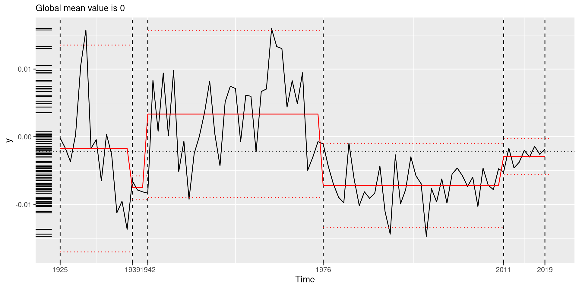
Ex. 1B: Modeling-defined eras

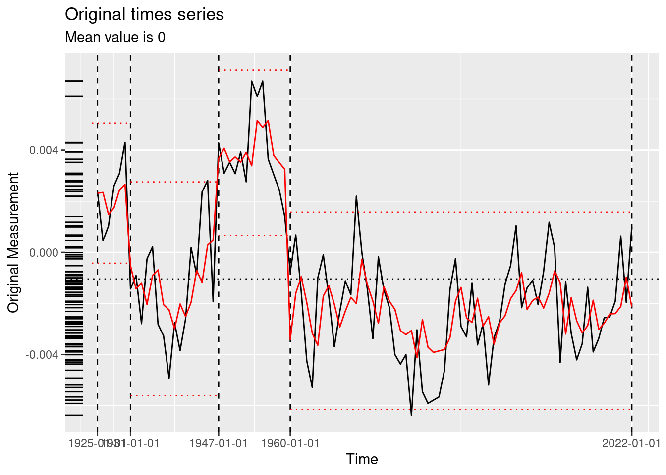
Ex. 2: Particulate matter in Bogotá

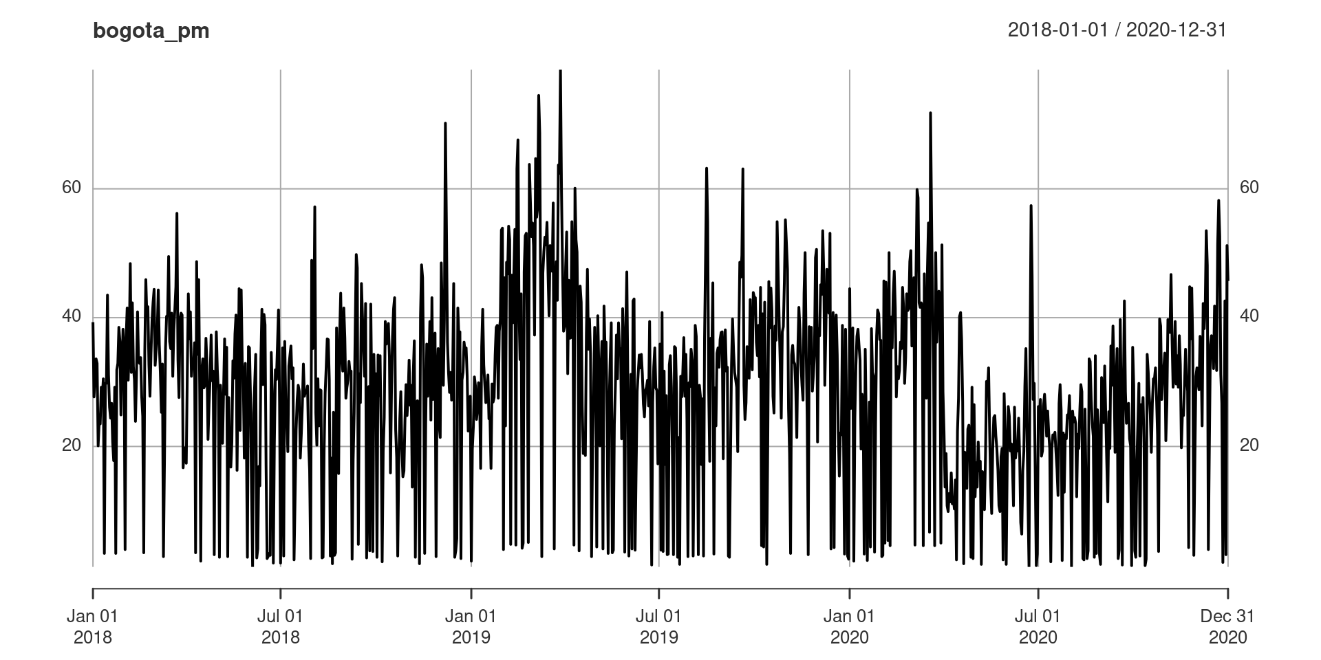
• True changepoints are unknown
• Can we find them??

What constitutes a solution?

Every solution includes three components:

• An algorithm to search the space (e.g., PELT, Binary segmentation, etc.)
• A (parametric) model to describe the data-generating process
• A penalized objection function to be optimized

Current state-of-the-art algorithms

• PELT (Killick, 2012)
  • polynomial time, exact solution
  • mild conditions
• Genetic algorithms (e.g., Shi, 2022)
  • flexible, but heuristic and can be slow
• Other approaches
  • Bayesian methods
  • Coen’s algorithm (Suárez-Sierra, et al., 2023)

Models

• For now, parametric: \(M(y | \theta)\)
• Given the data \(y\) and changepoint set \(\tau\), find optimal \(\hat{\theta}_\tau\)
• Ex: “meanshift” model:
  • regional means (\(\mu_i\)), national variance (\(\sigma^2\))
  • \(\theta = \{ \sigma^2, \mu_0, \ldots, \mu_m \}\)
  • Normal distribution

Penalized objective function: BIC

• Bayesian Information Criterion (BIC)
• \(k_M(\tau)\) is the number of parameters estimated by the model

\[ BIC(\tau, M(y|\hat{\theta}_\tau)) = \underbrace{k_M(\tau) \ln{n}}_{\text{penalty}} - 2 \ln{\underbrace{L_M(y | \hat{\theta}_\tau)}_{\text{likelihood}}}, \]

Penalized objective function: MDL

• Minimum Descriptive Length (MDL)
• \(a(\theta)\) is the number of regional parameters
• \(b(\theta)\) is the number of national parameters

\[ \begin{aligned} P_{MDL}(\tau) &= \frac{a(\theta_\tau)}{2} \cdot \sum_{j=0}^m \log{(\tau_{j+1} - \tau_j)} + 2 \ln{m} \\ &+ \sum_{j=2}^m \ln{\tau_j} + \left( 2 + b(\theta_\tau) \right) \ln{n} \end{aligned} \]

PELT software implementation

• changepoint package
• includes several (but not all) models
• includes several (but not all) penalty functions

Genetic algorithms software implementation

• 🆕 changepointGA package
• GA package can be customized (foreshadowing…)

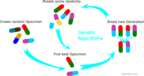
Other software implementations

• Many other packages (e.g., wbs, segmented, strucchange, qcc, bcp, ggchangepoint, etc.)…

Problems with the state-of-the-art

• a lot of different packages
• a lot of different interfaces
• a lot of different return objects
• not all algorithms work with all models or penalty functions

tidychangepoint

Introducing tidychangepoint

library(tidychangepoint)

• Joint work with Biviana Marcela Suárez Sierra (Universidad EAFIT)
• tidychangepoint

This paper compiles the change point detection mechanisms of several methods, such as PELT, WBS, ggchangepoint, BCP, and QCC, among others. Each of these methods has its own library in CRAN. We implement visual tools and comparative metrics for each method, so that Tidychangepoint users can select the model that best fits their observations.

Universidad

What does tidychangepoint do?

• wraps functions from existing packages
• syntax that is compatible with tidyverse
• comprehensive architecture in a single package
• incorporating:
  • new changepoint detection algorithms
  • new parametric models
  • new penalty functions

Using segment()

• segment() wraps a variety of CDP algorithms

mlb_pelt <- mlb_bavg |>
  segment(method = "pelt", penalty = "BIC")
class(mlb_pelt)

[1] "tidycpt"

names(mlb_pelt)

[1] "segmenter"    "model"        "elapsed_time" "time_index"  

Recovering changepoints

• Use changepoints() to recover the changepoint sets

changepoints(mlb_pelt)

[1] 15 18 52 87

changepoints(mlb_pelt, use_labels = TRUE) |>
  as_year()

[1] "1939" "1942" "1976" "2011"

Visualize the changepoint set

plot(mlb_pelt, use_time_index = TRUE)

Recover estimated parameters

tidy(mlb_pelt)

# A tibble: 5 × 10
  region  num_obs      min       max     mean       sd begin   end param_mu
  <chr>     <int>    <dbl>     <dbl>    <dbl>    <dbl> <dbl> <dbl>    <dbl>
1 [1,15)       14 -0.0137   0.0158   -0.00173 0.00779      1    15 -0.00173
2 [15,18)       3 -0.00813 -0.00650  -0.00750 0.000872    15    18 -0.00750
3 [18,52)      34 -0.00923  0.0160    0.00335 0.00628     18    52  0.00335
4 [52,87)      35 -0.0147  -0.000943 -0.00719 0.00315     52    87 -0.00719
5 [87,96)       9 -0.00518 -0.00142  -0.00290 0.00135     87    96 -0.00290
# ℹ 1 more variable: param_sigma_hatsq <dbl>

Recover model fit information

glance(mlb_pelt)

# A tibble: 1 × 8
  pkg      version algorithm seg_params model_name criteria fitness elapsed_time
  <chr>    <pckg_> <chr>     <list>     <chr>      <chr>      <dbl> <drtn>      
1 changep… 2.3     PELT      <list [1]> meanvar    BIC        -782. 0.072 secs  

Models provided

• Previously, “meanshift” model:
  • regional means (\(\mu_i\)), national variance (\(\sigma^2\))
  • \(\theta = \{ \sigma^2, \mu_0, \ldots, \mu_m \}\)
  • fit_meanshift_norm()

 [1] "fit_lmshift"            "fit_lmshift_ar1"        "fit_meanshift"         
 [4] "fit_meanshift_lnorm"    "fit_meanshift_norm"     "fit_meanshift_norm_ar1"
 [7] "fit_meanvar"            "fit_nhpp"               "fit_trendshift"        
[10] "fit_trendshift_ar1"    

Experiment with different models

compare_models(mlb_pelt)

# A tibble: 8 × 12
  pkg   version algorithm params num_cpts    rmse logLik   AIC   BIC  MBIC   MDL
  <chr> <pckg_> <chr>     <list>    <int>   <dbl>  <dbl> <dbl> <dbl> <dbl> <dbl>
1 tidy… 1.0.0.… meanshif… <dbl>         4 0.00507  367.  -714. -689. -689. -682.
2 tidy… 1.0.0.… meanshif… <dbl>         4 0.00490  367.  -711. -683. -688. -677.
3 tidy… 1.0.0.… trendshi… <dbl>         4 0.00472  374.  -718. -680. -703. -683.
4 tidy… 1.0.0.… splinesh… <dbl>         4 0.00439  381.  -722. -671. -717. -684.
5 tidy… 1.0.0.… meanvar   <NULL>        4 0.00507  367.  -706. -671. -689. -674.
6 tidy… 1.0.0.… meanvar   <NULL>        4 0.00507  367.  -706. -671. -689. -674.
7 tidy… 1.0.0.… trendshi… <dbl>         4 0.00465  372.  -711. -670. -698. -673.
8 tidy… 1.0.0.… nhpp      <dbl>         4 0.00507  -59.3  149.  187.  163.  184.
# ℹ 1 more variable: BMDL <dbl>

Try a different penalty

mlb_bavg |>
  segment(method = "pelt", penalty = "MBIC") |>
  plot(use_time_index = TRUE)

Try a different model

mlb_bavg |>
  segment(method = "pelt", model_fn = fit_meanshift_norm) |>
  plot(use_time_index = TRUE)

Try a different algorithm

mlb_bavg |>
  segment(method = "ga-shi", maxiter = 500, run = 50) |>
  plot(use_time_index = TRUE)

Roll your own genetic algorithm

mlb_bavg |>
  segment(
    method = "ga",
    model_fn = fit_trendshift_ar1, 
    penalty_fn = MDL,
    popSize = 500,
    maxiter = 10000, 
    run = 50
  )

• tidychangepoint includes more than 10 models and 5 penalty functions
• More can be user-defined!

Diagnose the model fit

Learn more

• Package documentation
• GitHub repository
• Paper draft
• arXiv draft

Thank you!!!