04: Center, Shape, and Spread
IMS, Ch. 4–5
Feb 4, 2026
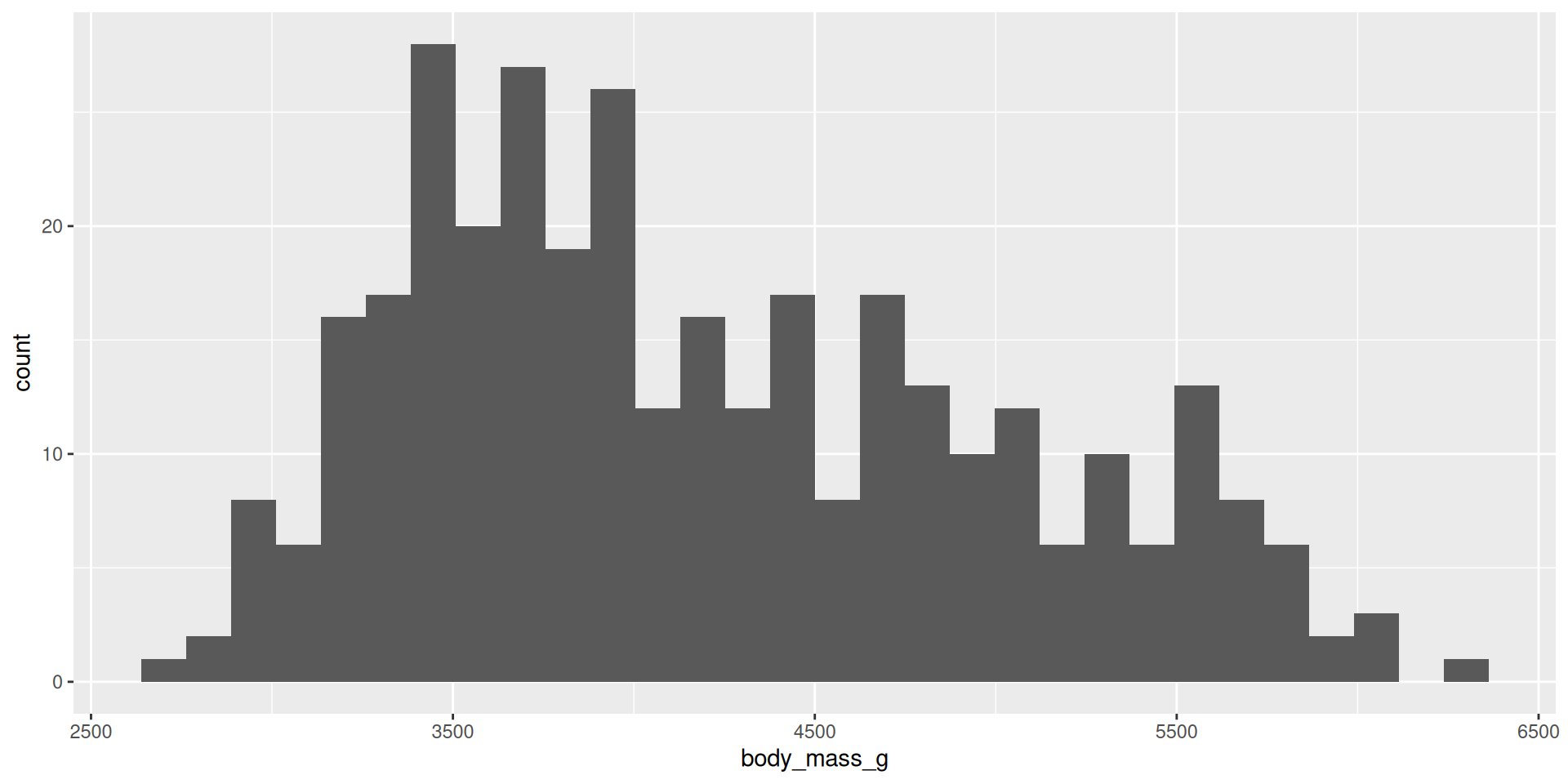
Histogram
Summarize the shape of the distribution of one variable
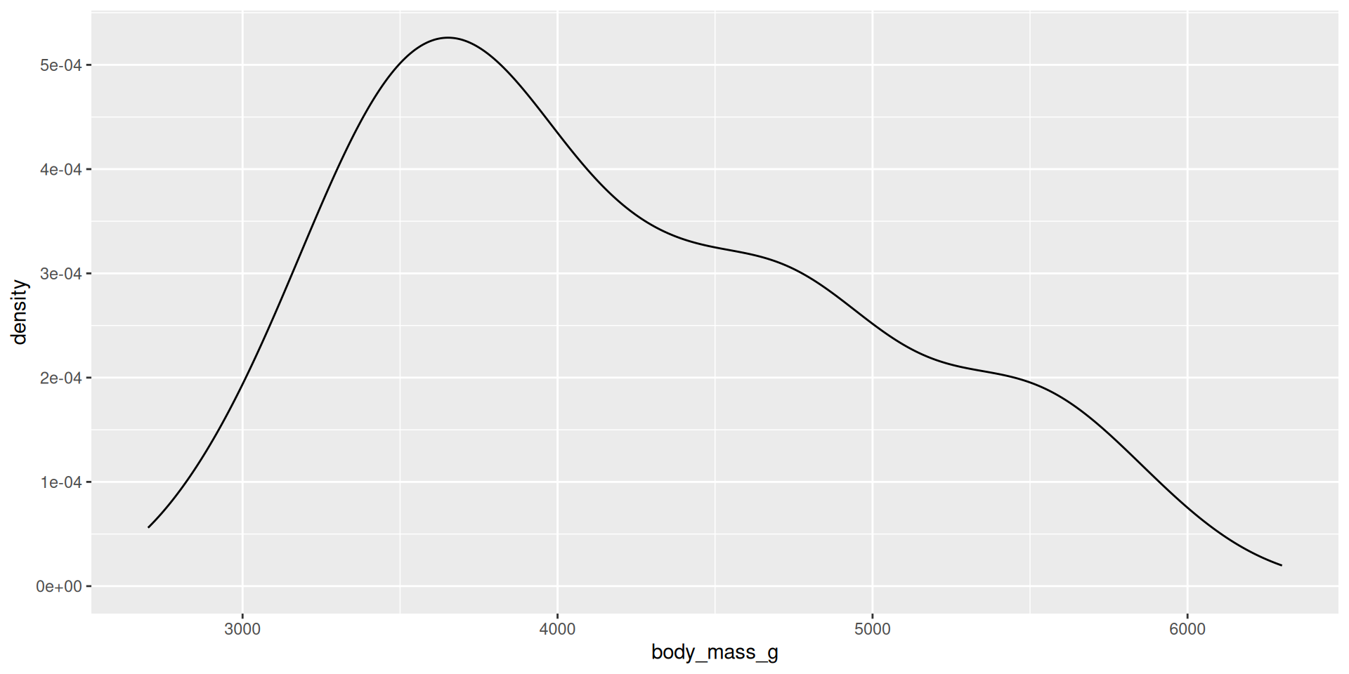
Density plot
Summarize the shape of the distribution of one variable
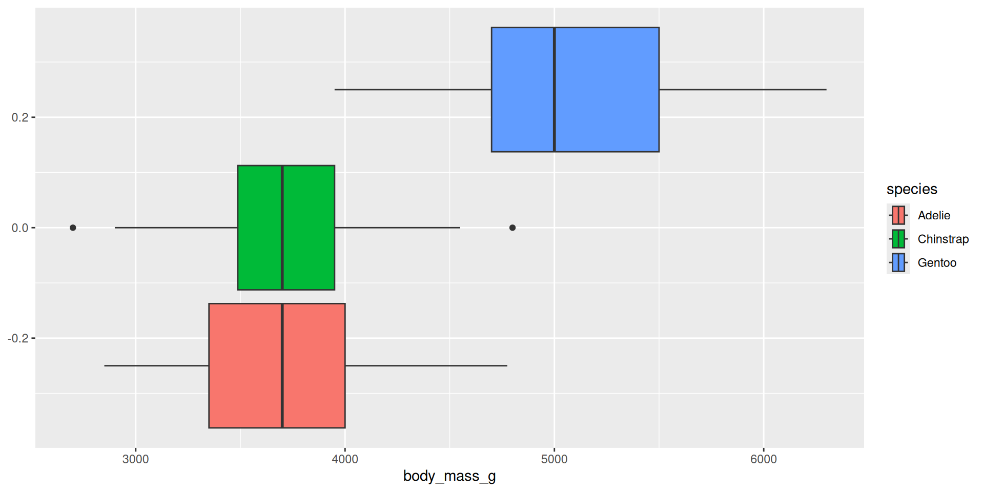
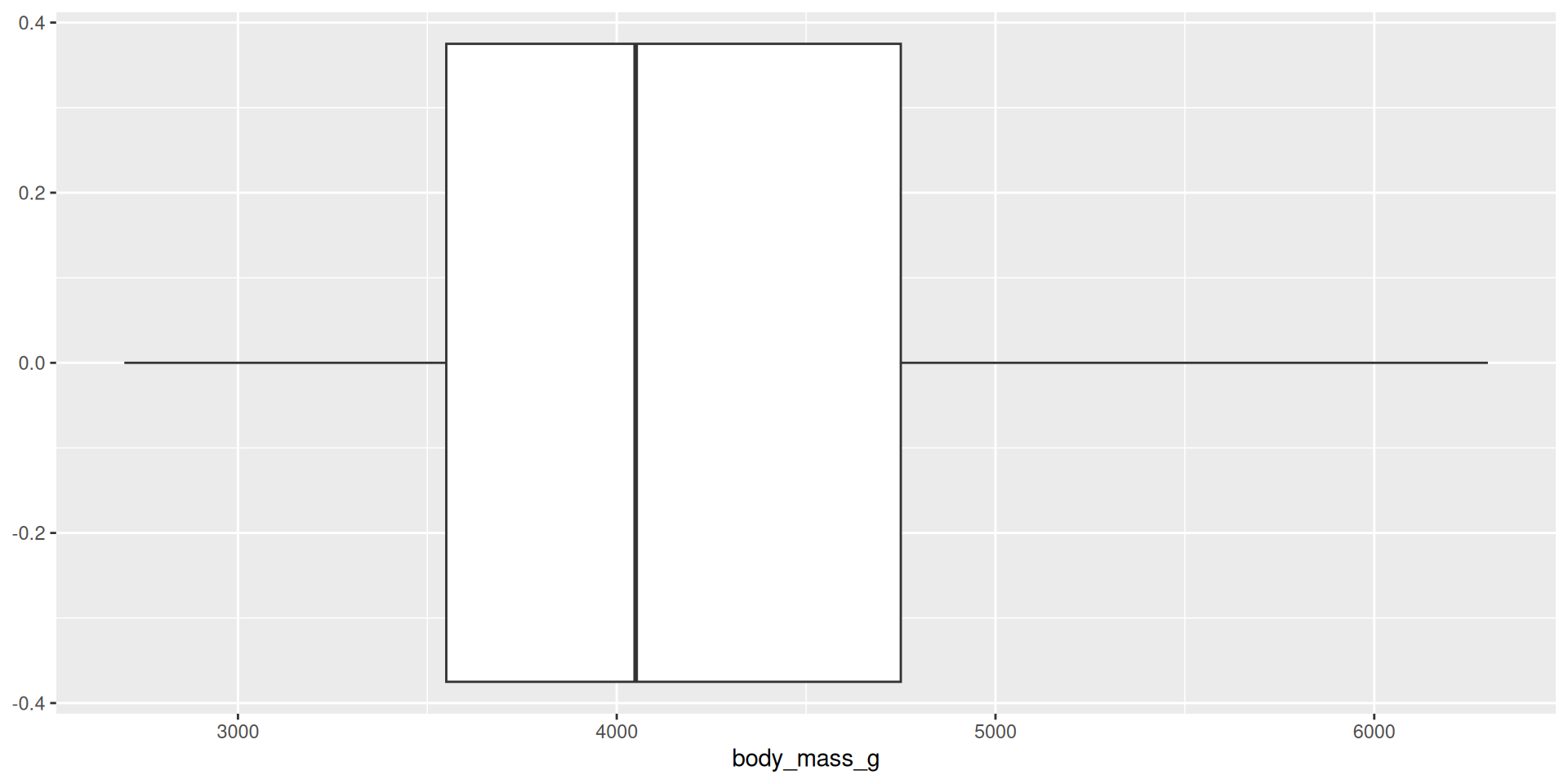
Box plot
Summarize the shape of the distribution of one variable
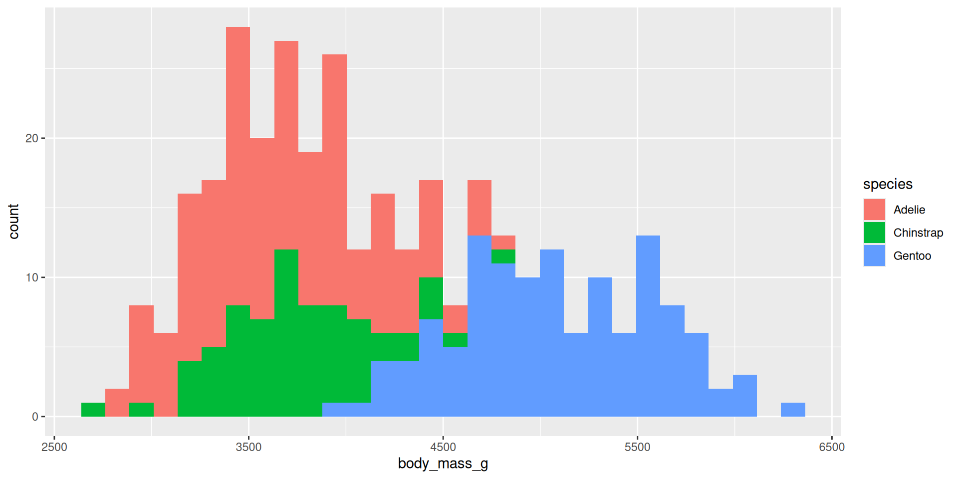
Histogram: two variables
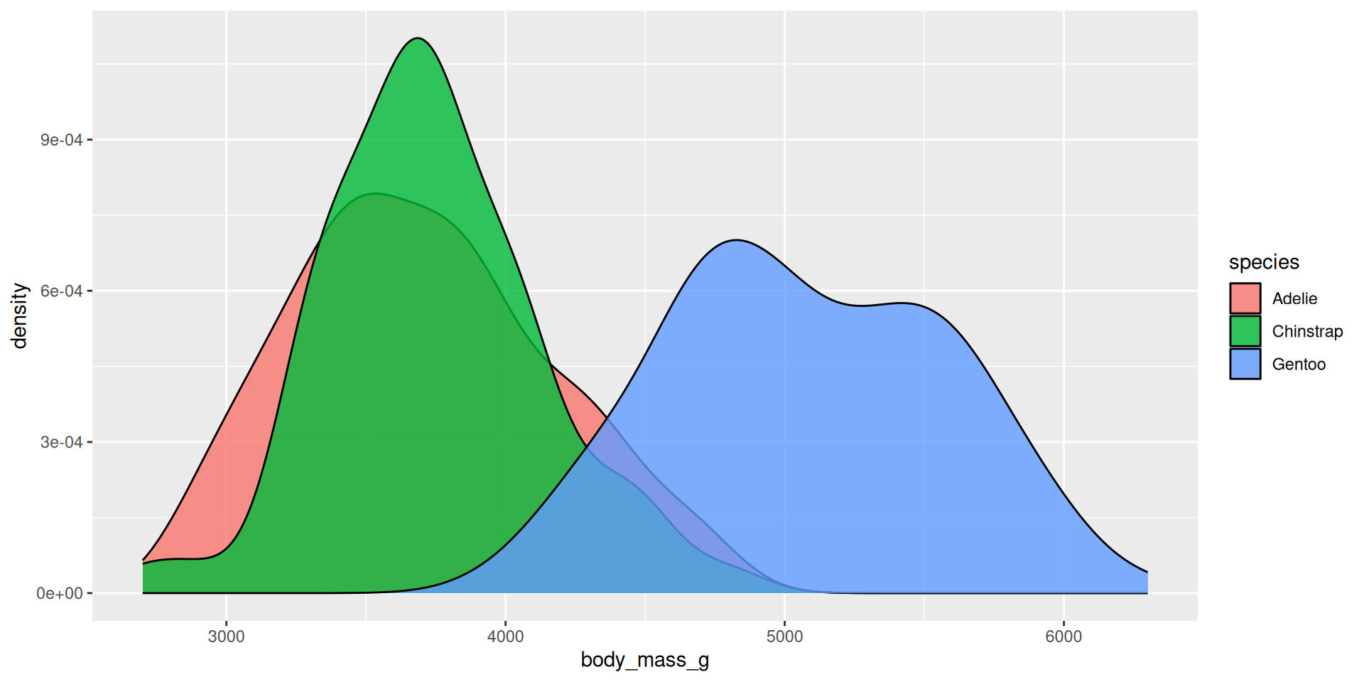
Density plot: two variables
Boxplot: two variables