Stratified sampling demo

Authors

Affiliation

Stratified sampling simulation

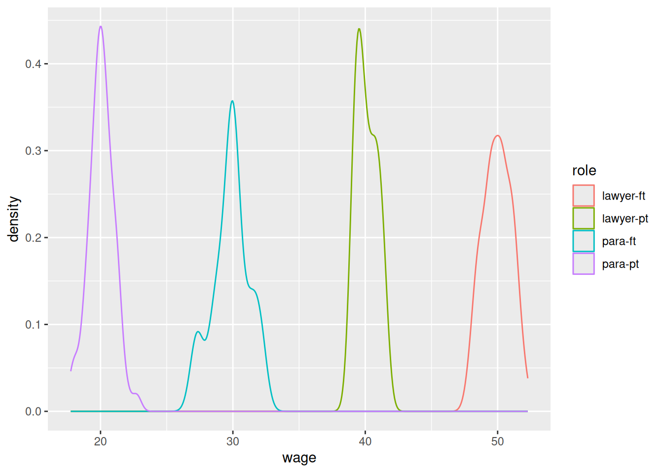
Recall the stratified sampling exercise from last time, and suppose that hourly wages were normally distributed with means $50, $40, $30, and $20, among the 90 lawyers working full-time, 18 lawyers working part-time, 9 paralegals working full-time, and 63 paralegals working part-time, respectively. The following R code builds a data frame that represents one possible reality.

library(tidyverse)
staff <- tibble(
  role = c(
    rep("lawyer-ft", 90), 
    rep("lawyer-pt", 18), 
    rep("para-ft", 9), 
    rep("para-pt", 63)
  ),
  wage = c(
    rnorm(90, mean = 50), 
    rnorm(18, 40), 
    rnorm(9, 30), 
    rnorm(63, 20)
  )
)
staff

# A tibble: 180 × 2
   role       wage
   <chr>     <dbl>
 1 lawyer-ft  50.9
 2 lawyer-ft  50.3
 3 lawyer-ft  51.7
 4 lawyer-ft  50.7
 5 lawyer-ft  51.1
 6 lawyer-ft  49.3
 7 lawyer-ft  51.2
 8 lawyer-ft  49.9
 9 lawyer-ft  50.2
10 lawyer-ft  49.4
# ℹ 170 more rows

Note that wages are similar within the four groups, but dissimilar among the groups. This command will draw separate densities for the four groups on the same plot.

ggplot(data = staff, aes(x = wage, color = role)) +
  geom_density()

We want to estimate the mean wage among all 180 workers. In this case, since we know the wage of all of the workers, we can just compute it.

actual <- staff |>
  summarize(
    number_of_employees = n(),
    mean_wage = mean(wage)
  )
actual

# A tibble: 1 × 2
  number_of_employees mean_wage
                <int>     <dbl>
1                 180      37.5

But recall that for the purposes of this exercise, we’re supposing we don’t actually know all 180 wages, and we are asked to sample 40 of them.

Simple random sampling

We can take a simple random sample and compute the mean wage within that sample.

# simple random sampling
staff |>
  sample_n(40) |>
  summarize(
    number_of_employees = n(),
    mean_wage = mean(wage)
  )

# A tibble: 1 × 2
  number_of_employees mean_wage
                <int>     <dbl>
1                  40      39.9

Note that this is close to the actual mean wage, but not the same. Note also that each time we take a different random sample, we get a different mean wage in that sample.

Stratified sampling

Now let’s implement the stratified sampling scheme.

# Stratified sampling
strat_sample <- staff |>
  group_by(role) |>
  group_split() |>
  map2(c(20, 4, 2, 14), sample_n) |>
  bind_rows()

strat_sample |>
  summarize(
    number_of_employees = n(),
    mean_wage = mean(wage)
  )

# A tibble: 1 × 2
  number_of_employees mean_wage
                <int>     <dbl>
1                  40      37.7

Again, the stratified sample mean is close to the actual value, but not the same. It will also differ each time we take a different random sample. So why might we prefer stratified sampling over simple random sampling?

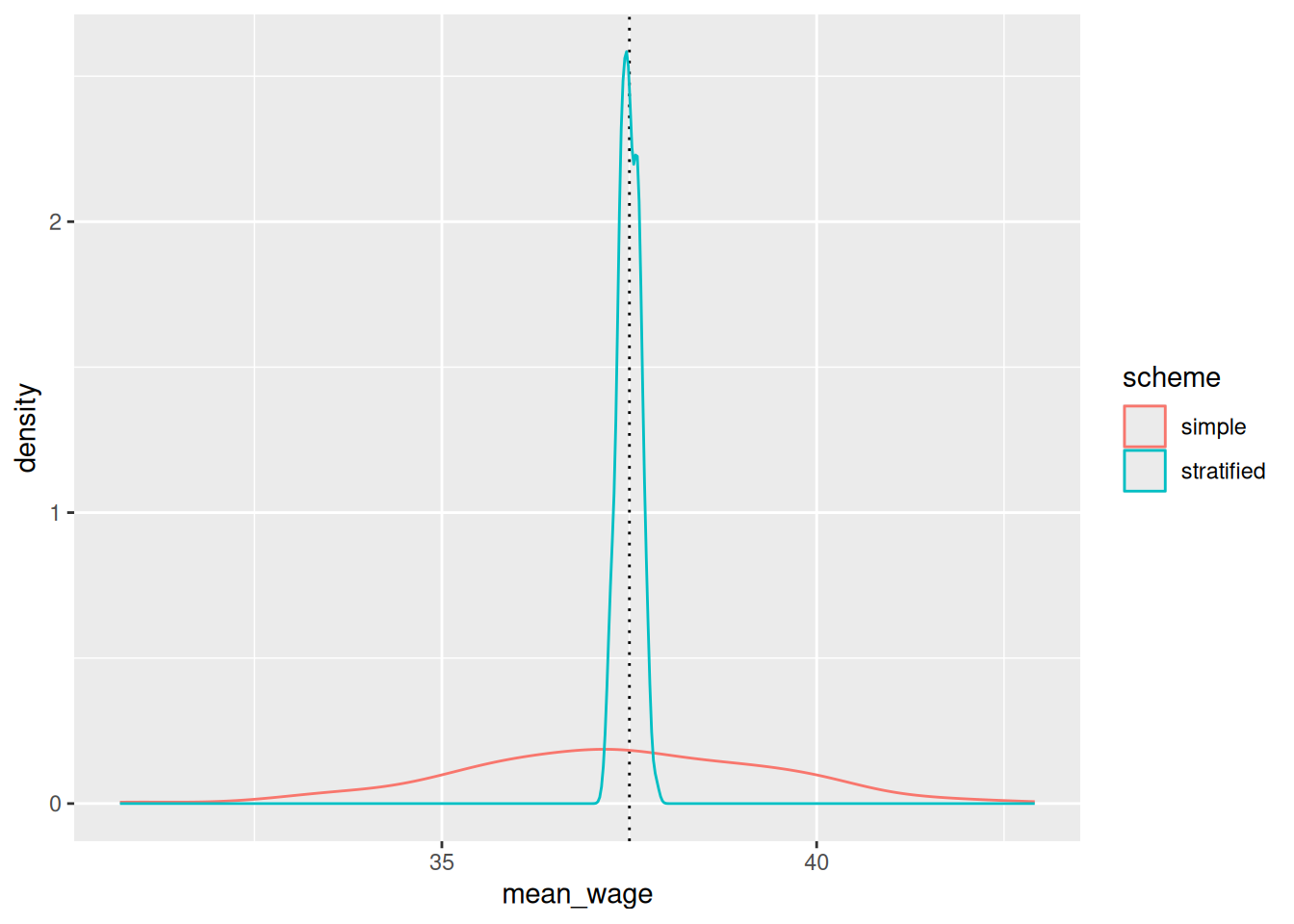
Sampling distributions

Let’s compare the distribution of sample means if we do this many, many times!

# Comparison
num_trials <- 250

null_dist_srs <- 1:num_trials |>
  map(~staff |>
    sample_n(40) |>
    summarize(
      number_of_employees = n(),
      mean_wage = mean(wage)
    )
) |>
  bind_rows() |>
  mutate(scheme = "simple")

null_dist_strat <- 1:num_trials |>
  map(~staff |>
    group_split(role) |>
    map2(c(20, 4, 2, 14), sample_n) |>
    bind_rows() |>
    summarize(
      number_of_employees = n(),
      mean_wage = mean(wage)
    )
) |>
  bind_rows() |>
  mutate(scheme = "stratified")

sim <- bind_rows(null_dist_srs, null_dist_strat)

Visualize the null distributions.

ggplot(
  data = sim, 
  aes(x = mean_wage, color = scheme)
) + 
  geom_vline(xintercept = pull(actual, mean_wage), linetype = 3) +
  geom_density()