In-class scratch work

Authors

Affiliation

1/28

library(tidyverse)
library(palmerpenguins)
penguins

# A tibble: 344 × 8
   species island    bill_length_mm bill_depth_mm flipper_length_mm body_mass_g
   <fct>   <fct>              <dbl>         <dbl>             <int>       <int>
 1 Adelie  Torgersen           39.1          18.7               181        3750
 2 Adelie  Torgersen           39.5          17.4               186        3800
 3 Adelie  Torgersen           40.3          18                 195        3250
 4 Adelie  Torgersen           NA            NA                  NA          NA
 5 Adelie  Torgersen           36.7          19.3               193        3450
 6 Adelie  Torgersen           39.3          20.6               190        3650
 7 Adelie  Torgersen           38.9          17.8               181        3625
 8 Adelie  Torgersen           39.2          19.6               195        4675
 9 Adelie  Torgersen           34.1          18.1               193        3475
10 Adelie  Torgersen           42            20.2               190        4250
# ℹ 334 more rows
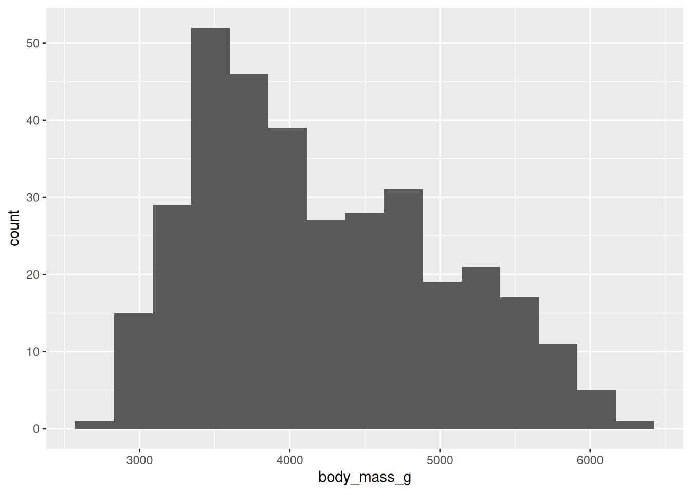
# ℹ 2 more variables: sex <fct>, year <int>

ggplot(data = penguins, mapping = aes(x = body_mass_g)) +
  geom_histogram(bins = 15)

Warning: Removed 2 rows containing non-finite outside the scale range
(`stat_bin()`).

ggplot(data = starwars, aes(x = height, color = "red")) +
  geom_density()

Warning: Removed 6 rows containing non-finite outside the scale range
(`stat_density()`).

starwars |>
  summarize(mean_height = mean(height, na.rm = FALSE))

# A tibble: 1 × 1
  mean_height
        <dbl>
1          NA

2/6

library(tidyverse)
# number of players
n_nba <- 32 * 12
n_wnba <- 15 * 12

players <- tibble(
  league = c(rep("nba", times = n_nba), rep("wnba", times = n_wnba)),
  height = c(
    rnorm(n_nba, mean = 78, sd = 10.5), 
    rnorm(n_wnba, mean = 72, sd = 1)
  )
)

players |> 
  head()

# A tibble: 6 × 2
  league height
  <chr>   <dbl>
1 nba      80.5
2 nba      81.6
3 nba      82.8
4 nba      72.0
5 nba      82.2
6 nba     100. 

ggplot(players, aes(x = height)) +
  geom_density(alpha = 0.8)

library(openintro)

Loading required package: airports

Loading required package: cherryblossom

Loading required package: usdata

ggplot(babies, aes(x = gestation, y = bwt)) +
  geom_point() +
  scale_x_continuous("Length of Gestation (days)") +
  scale_y_continuous("Birthweight (ounces)")

Warning: Removed 13 rows containing missing values or values outside the scale range
(`geom_point()`).

sw2 <- starwars |>
  filter(mass < 200)

ggplot(sw2, aes(x = height, y = mass)) + geom_point()

ggplot(babies, aes(x = smoke, y = bwt)) +
  geom_jitter(width = 0.05, alpha = 0.1)

Warning: Removed 10 rows containing missing values or values outside the scale range
(`geom_point()`).

ggplot(babies, aes(x = factor(parity), y = bwt)) +
  geom_boxplot()

2/9

library(mosaic)
head(RailTrail)

  hightemp lowtemp avgtemp spring summer fall cloudcover precip volume weekday
1       83      50    66.5      0      1    0        7.6   0.00    501    TRUE
2       73      49    61.0      0      1    0        6.3   0.29    419    TRUE
3       74      52    63.0      1      0    0        7.5   0.32    397    TRUE
4       95      61    78.0      0      1    0        2.6   0.00    385   FALSE
5       44      52    48.0      1      0    0       10.0   0.14    200    TRUE
6       69      54    61.5      1      0    0        6.6   0.02    375    TRUE
  dayType
1 weekday
2 weekday
3 weekday
4 weekend
5 weekday
6 weekday

ggplot(RailTrail, aes(y = volume, x = avgtemp)) +
  geom_point() +
  geom_smooth(method = "lm", se=0)

RailTrail|>
  summarize(r=cor(avgtemp,volume))

          r
1 0.4268535

lm(volume~avgtemp,data=RailTrail)

Call:
lm(formula = volume ~ avgtemp, data = RailTrail)

Coefficients:
(Intercept)      avgtemp  
     99.602        4.802  

2/11

library(usdata)
lm(poverty ~ unempl, data = state_stats) |>
  summary()

Call:
lm(formula = poverty ~ unempl, data = state_stats)

Residuals:
    Min      1Q  Median      3Q     Max 
-5.1974 -1.8006 -0.2719  1.9045  6.6224 

Coefficients:
            Estimate Std. Error t value Pr(>|t|)    
(Intercept)   9.2528     1.7107   5.409 1.88e-06 ***
unempl        0.5605     0.2216   2.529   0.0147 *  
---
Signif. codes:  0 '***' 0.001 '**' 0.01 '*' 0.05 '.' 0.1 ' ' 1

Residual standard error: 2.873 on 49 degrees of freedom
Multiple R-squared:  0.1155,    Adjusted R-squared:  0.09745 
F-statistic: 6.398 on 1 and 49 DF,  p-value: 0.01469

1 - 404/457

[1] 0.1159737

2/16

library(tidyverse)
library(mosaic)
lm(volume ~ weekday, data = RailTrail) |>
  summary()

Call:
lm(formula = volume ~ weekday, data = RailTrail)

Residuals:
     Min       1Q   Median       3Q      Max 
-301.714  -91.419    5.081   80.831  305.286 

Coefficients:
            Estimate Std. Error t value Pr(>|t|)    
(Intercept)   430.71      23.16  18.598  < 2e-16 ***
weekdayTRUE   -80.29      27.90  -2.878  0.00503 ** 
---
Signif. codes:  0 '***' 0.001 '**' 0.01 '*' 0.05 '.' 0.1 ' ' 1

Residual standard error: 122.5 on 88 degrees of freedom
Multiple R-squared:  0.08601,   Adjusted R-squared:  0.07562 
F-statistic: 8.281 on 1 and 88 DF,  p-value: 0.005028

library(tidyverse)
nyc <- read_csv("https://gattonweb.uky.edu/faculty/sheather/book/docs/datasets/nyc.csv")

Rows: 168 Columns: 7
── Column specification ────────────────────────────────────────────────────────
Delimiter: ","
chr (1): Restaurant
dbl (6): Case, Price, Food, Decor, Service, East

ℹ Use `spec()` to retrieve the full column specification for this data.
ℹ Specify the column types or set `show_col_types = FALSE` to quiet this message.

ggplot(data = nyc, aes(x = Food, y = Price)) +
  geom_jitter(width = 0.1, alpha = 0.5, size = 2) + 
  geom_smooth(method = "lm", se = 0) +
  xlab("Jittered food rating") + 
  ylab("Average Price (US$)") +
  moderndive::geom_parallel_slopes(aes(color = factor(East)), se = 0)

`geom_smooth()` using formula = 'y ~ x'

mod <- lm(Price ~ Food + East, data = nyc)

2/18

mod_decor <- lm(Price ~ Decor + East, data = nyc)

mod_decor

Call:
lm(formula = Price ~ Decor + East, data = nyc)

Coefficients:
(Intercept)        Decor         East  
     -2.962        2.471        3.090  

lm(Price ~ Food + Service, data = nyc)

Call:
lm(formula = Price ~ Food + Service, data = nyc)

Coefficients:
(Intercept)         Food      Service  
    -21.159        1.495        1.704  

3/6

sample(1:6, size = 100000, replace = TRUE) |>
  mean()

[1] 3.50324

3/9

library(tidyverse)
library(googlesheets4)
gs4_deauth()
dice <- read_sheet("https://docs.google.com/spreadsheets/d/1FvmWcm0ObURhJl9KhwNIM5sKMsbyFoF1Wie7fU6P_Sk/") |>
  mutate(id = row_number())

✔ Reading from "sds210-s26-sampling".

✔ Range 'Sheet1'.

dice

# A tibble: 35 × 6
       X     Y     Z     W color    id
   <dbl> <dbl> <dbl> <dbl> <chr> <int>
 1   6     6      10    10 black     1
 2   6     6      10    10 black     2
 3   5.7   6       9     9 black     3
 4   3.6   3.5     4     1 white     4
 5   5.1   6       9     7 black     5
 6   5.9   6       9     9 black     6
 7   5.7   6       9     9 black     7
 8   6     6      10    10 black     8
 9   5.6   6      10     9 black     9
10   3.2   4       5     2 white    10
# ℹ 25 more rows

dice |>
  group_by(color) |>
  summarize(
    x_bar = mean(X, na.rm = TRUE),
    y_bar = mean(Y),
    z_bar = mean(Z),
    w_bar = mean(W),
  )

# A tibble: 2 × 5
  color x_bar y_bar z_bar w_bar
  <chr> <dbl> <dbl> <dbl> <dbl>
1 black  5.57  5.91  9.48  8.30
2 white  3.54  3.71  4.83  1.92

dice |>
  pivot_longer(-c(color, id), names_to = "r_v", values_to = "value") |>
ggplot(aes(x = value, fill = color)) +
  geom_histogram() +
  facet_wrap(vars(r_v))

`stat_bin()` using `bins = 30`. Pick better value `binwidth`.

3/11

library(tidyverse)
library(openintro)
ebola_survey

# A tibble: 1,042 × 1
   quarantine
   <fct>     
 1 favor     
 2 favor     
 3 favor     
 4 favor     
 5 favor     
 6 against   
 7 favor     
 8 favor     
 9 favor     
10 favor     
# ℹ 1,032 more rows

library(infer)

Attaching package: 'infer'

The following objects are masked from 'package:mosaic':

    prop_test, t_test

p_hat <- ebola_survey |>
  specify(response = quarantine, success = "favor") |>
  calculate(stat = "prop")
p_hat

Response: quarantine (factor)
# A tibble: 1 × 1
   stat
  <dbl>
1 0.820

ebola_survey |>
  specify(response = quarantine, success = "favor") |>
  generate(1000, method = "bootstrap") |>
  calculate(stat = "prop") |>
  get_ci()

Setting `type = "bootstrap"` in `generate()`.

# A tibble: 1 × 2
  lower_ci upper_ci
     <dbl>    <dbl>
1    0.797    0.842

ebola_survey |>
  specify(response = quarantine, success = "favor") |>
  generate(1000, method = "bootstrap") |>
  calculate(stat = "prop") |>
  visualize()

Setting `type = "bootstrap"` in `generate()`.