# A tibble: 1 × 4
  yearID     N mean_BAvg sd_BAvg
   <int> <int>     <dbl>   <dbl>
1 1980 148 0.279 0.0276Inference for a difference in proportions
IMS, Ch. 17
Smith College
Apr 8, 2026
Recap
Inference for a single proportion
| Method | null dist. | sampling dist. |
|---|---|---|
| 1: probability | scaled \(Binom(n, p_0)\) | scaled \(Binom(n, \hat{p})\) |
| 2: simulation | parametric bootstrap (centered at \(p_0\)) | bootstrap (centered at \(\hat{p}\)) |
| 3: normal approx. | \(N \left( p_0, \sqrt{\frac{p_0 (1 - p_0)}{n}} \right)\) | \(N \left( \hat{p}, \sqrt{\frac{\hat{p} (1 - \hat{p})}{n}} \right)\) |
Applying the Normal Model
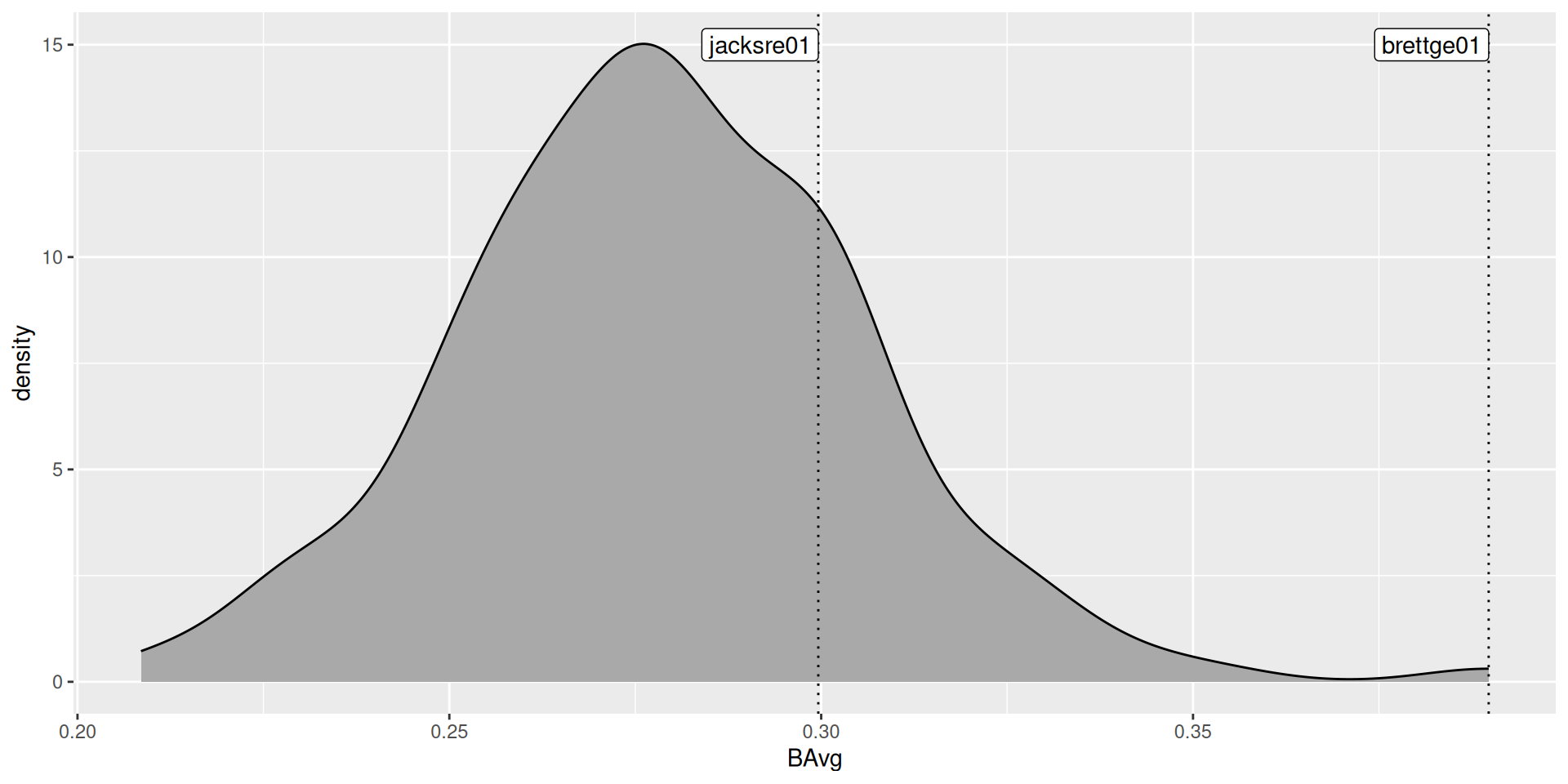
Baseball
Recall the baseball example from last time
George Brett
George Brett, who hit .390 in 1980, won the AL MVP.

Reggie Jackson
The player who finished second in the balloting, Reggie Jackson, hit .300 (with 41 home runs).

Get the data
The truth
Use the actual batting averages from the 148 players with at least 400 at-bats:
True sampling distribution?
Normal approximation
- Assume that batting average is distributed normally and use the observed mean and standard deviation to specify the distribution:
Normal approximation
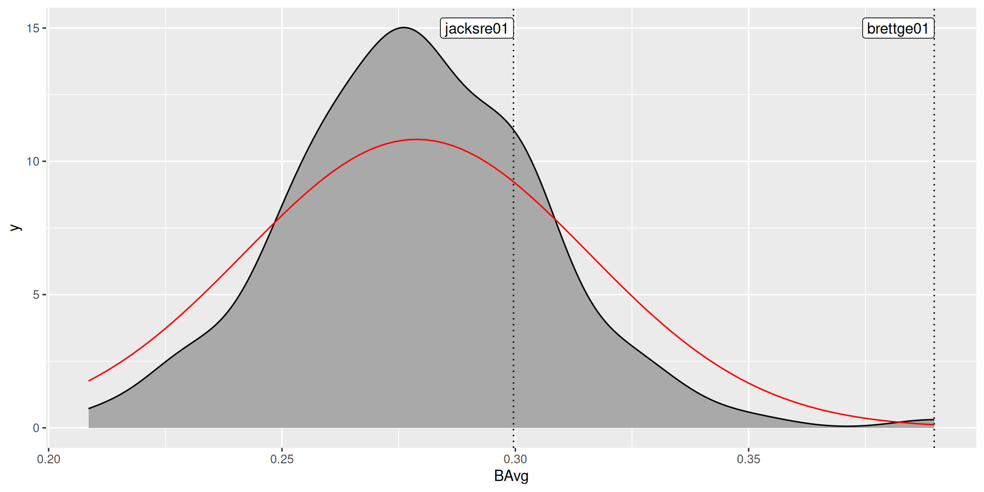
Your turn
Was the normal approximation appropriate? Why or why not?
Review the CLT
Difference of two proportions
Inference for two proportions
| Method | null dist. | sampling dist. |
|---|---|---|
| 1: probability | ? | ? |
| 2: simulation | randomization test (centered at \(0\)) | two bootstraps (centered at \(\hat{p}_1 - \hat{p}_2\)) |
| 3: normal approx. | \(N(0, SE_{pool})\) | \(N \left( \hat{p}_1 - \hat{p}_2, SE_{\hat{p}_1 - \hat{p}_2} \right)\) |
- See IMS, Chapter 17
Standard errors
- \(SE_{pool}\):
\[ \hat{p}_{pool} = \frac{\hat{p}_1 n_1 + \hat{p}_2 n_2}{n_1 + n_2} = \frac{n_1}{n_1 + n_2} \cdot \hat{p}_1 + \frac{n_2}{n_1 + n_2} \cdot \hat{p}_2 \\ SE_{pool} = \sqrt{ \hat{p}_{pool} (1 - \hat{p}_{pool}) \left( \frac{1}{n_1} + \frac{1}{n_2} \right) } \]
- \(SE_{\hat{p}_1 - \hat{p}_2}\):
\[ SE_{\hat{p}_1 - \hat{p}_2} = \sqrt{\frac{\hat{p}_1 (1 - \hat{p}_1)}{n_1} + \frac{\hat{p}_2 (1 - \hat{p}_2)}{n_2}} \]
Where does that come from?
Suppose we have \(X \sim Binom(n_1, p_1)\) and \(Y \sim Binom(n_2, p_2)\).
- Define a new random variable \(Z\):
\[ Z = \frac{X}{n_1} - \frac{Y}{n_2} \]
\[ \mathbb{E}[Z] = \frac{\mathbb{E}[X]}{n_1} - \frac{\mathbb{E}[Y]}{n_2} = \frac{n_1 p_1}{n_1} - \frac{n_2 p_2}{n_2} = p_1 - p_2 \]
And so the variance…
\[ Var[Z] = \frac{p_1 (1-p_1)}{n_1} + \frac{p_2 (1-p_2)}{n_2} \]
- The standard error is
\[ SE_Z = SE_{ \hat{p}_1 - \hat{p}_2 } = \sqrt{SE_{\hat{p}_1}^2 + SE_{\hat{p}_2}^2 } \]
Conditions
Independence Condition
The data are independent within and between the two groups. Generally this is satisfied if the data come from two independent random samples or if the data come from a randomized experiment.
Success-failure condition
The success-failure condition holds for both groups, where we check successes and failures in each group separately. That is, we should have at least 10 successes and 10 failures in each of the two groups.
![]()