Central Limit Theorem and the Normal Distribution

IMS, Ch. 13

Benjamin S. Baumer

Smith College

Mar 30, 2026

Recall the Three Methods for constructing a sampling distribution

Central Limit Theorem

Central Limit Theorem

Central Limit Theorem

• The distribution of the sample mean (i.e., the sampling distribution of the mean) will be approximately normal for reasonably large \(n\) (e.g., at least 30)

• Provides a mathematical approximation to the simulated null distributions with which we have been working
• Consider the practical difficulties of simulating null distributions without a computer!

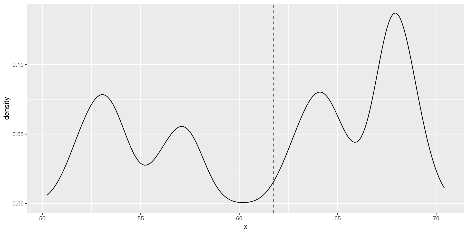
Simulation: a multimodal distribution

library(tidyverse)
n <- 1000
ds <- tibble(
  a = rnorm(n, mean = 53), 
  b = rnorm(n, mean = 57, sd = 0.8),
  c = rnorm(n, mean = 64), 
  d = rnorm(n, mean = 68, sd = 0.8), 
  p = runif(n)
  ) |>
  mutate(
    x = case_when(
      p < 0.25 ~ a, 
      p < 0.4 ~ b, 
      p < 0.65 ~ c,
      TRUE ~ d
    )
  )

pop_plot <- ggplot(
  data = ds, aes(x = x)
) +
  geom_density(adjust = 0.5) +
  geom_vline(aes(xintercept = mean(x)), linetype = 2)
pop_plot

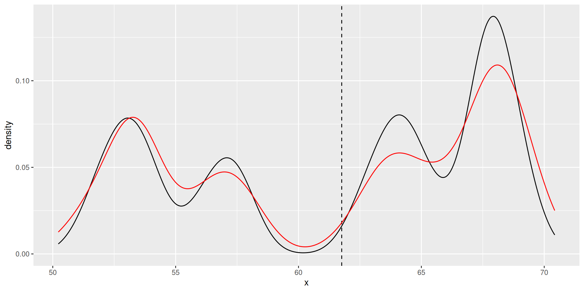
Simulation: sampling dist of the mean

draw <- function(data, n = 1) {
  data |>
    sample_n(n) |>
    summarize(
      mean = mean(x)
    )
}
sim <- 1:200 |>
  map(~draw(ds, n = 1)) |>
  bind_rows()

pop_plot + 
  geom_density(
    data = sim, aes(x = mean), 
    adjust = 0.5, color = "red"
  )

Normal distribution

Normal distribution

• Has two parameters: \(\mu\), \(\sigma\)

• Density function: \[ f(x; \mu, \sigma) = \frac{1}{\sqrt{2 \pi} \sigma} \exp \left( \frac{(x - \mu)^2}{2 \sigma^2} \right) \]

• \(N(0,1)\): Standard Normal distribution

Your turn

• Consider \(N(\mu, \sigma)\). What is the distribution of \(N(\mu, \sigma) - \mu\)?
• What is the distribution of \(N(0, \sigma)/ \sigma\)?
• If \(X \sim N(\mu, \sigma)\), then what is the distribution of \(Z = \frac{x - \mu}{\sigma}\)?

Example: z-score

SAT scores are distributed nearly normally with mean 1500 and sd 300. ACT scores are distributed nearly normally with mean 21 and sd 5. A college admissions officer wants to determine which of the two applicants scored better on their standardized test with respect to the other test takers: Brianna, who eared an 1800 on her SAT, or Doug, who scored a 24 on his ACT?

• Brianna’s score is \(\frac{1800-1500}{300} = 1\) sd above the mean.

• Doug’s score is \(\frac{24-21}{5} = 0.6\) sd above the mean.

The Empirical Rule

For any normally distributed variable

• About 68% is contained within 1 sd of the mean
• About 95% is contained within 2 sd of the mean
• About 99.7% is contained within 3 sd of the mean
• About 38% is contained within 0.5 standard deviations of the mean
  • The middle 38% of the distribution is about 1 sd wide

Sample Calculation

What percentage of the distribution is less than 2 standard deviations above the mean?

By the rule:

• About 95% of the population is within two standard deviations of the mean
• By symmetry, half of those are above the mean, and half below it
• Thus, we estimate that about \(95/2 = 47.5\%\) is less than 2 standard deviations above the mean

Sample Calculation

What percentage of the distribution is less than 2 standard deviations above the mean?

From the picture:

• The area is about \(34.1\% + 13.6\% = 47.7\%\)

Your turn

Assume that the distribution of heights of adult women is approximately normal with mean 64 inches and standard deviation 2.5 inches.

• What percentage of women are taller than 5’9”?
• Between what heights do the middle 95% of women fall?
• What percentage of women are shorter than 61.5 inches?
• A professor claims that about 51% of women are between 61.5 and 65.25 inches tall. Is this claim accurate?

Margin of error

• The distance given by \(z_{\alpha/2}^* \cdot SE\) is called the margin of error
• \(z_{\alpha/2}^*\) is the cutoff value found on the normal distribution
• Most commonly, \(z_{0.025}^*\) is 1.96

qnorm(c(0.025, 0.975))

[1] -1.959964  1.959964