# A tibble: 1,000 × 13
    fage  mage mature     weeks premie visits gained weight lowbirthweight sex
   <int> <dbl> <chr>      <dbl> <chr>   <dbl>  <dbl>  <dbl> <chr>          <chr>
 1    34    34 younger m…    37 full …     14     28   6.96 not low        male
 2    36    31 younger m…    41 full …     12     41   8.86 not low        fema…
 3    37    36 mature mom    37 full …     10     28   7.51 not low        fema…
 4    NA    16 younger m…    38 full …     NA     29   6.19 not low        male
 5    32    31 younger m…    36 premie     12     48   6.75 not low        fema…
 6    32    26 younger m…    39 full …     14     45   6.69 not low        fema…
 7    37    36 mature mom    36 premie     10     20   6.13 not low        fema…
 8    29    24 younger m…    40 full …     13     65   6.74 not low        male
 9    30    32 younger m…    39 full …     15     25   8.94 not low        fema…
10    29    26 younger m…    39 full …     11     22   9.12 not low        male
# ℹ 990 more rows
# ℹ 3 more variables: habit <chr>, marital <chr>, whitemom <chr>Inference for regression (testing)
IMS, Ch. 24
Smith College
Nov 30, 2022
Inference for regression
Inference for regression
| Method | null dist. | sampling dist. |
|---|---|---|
| 1: simulation | randomization test (entered at \(\beta_1 = 0\)) | bootstrap (centered at \(\hat{\beta}_1\)) |
| 2: probability | ? | ? |
| 3: \(t\)-approx. | \(t(d.f.)\) | \(t \left(d.f. \right)\) |
- See IMS, Chapter 24
Why inference for regression?
- Regression models have parameters (e.g., \(\beta_0, \beta_1\), etc.)
\[ Y = \beta_0 + \beta_1 \cdot X + \epsilon \, , \]
You know how to find \(\hat{\beta}_1\)
We can test hypotheses about \(\beta_1\) (i.e., \(\beta_1 = 0\))
We can find confidence intervals for \(\beta_1\)
Hypothesis testing
- We are particularly interested in testing the hypothesis that \(\beta_1 = 0\)
- We can do a randomization test
- Shuffle the response variable
- Or, use a \(t\)-based approximation:
- test statistic is: \(t_{\beta_1} = \frac{\hat{\beta}_1 - 0}{SE_{\hat{\beta}_1}}\)
- degrees of freedom is \((n-1) - (\text{# of predictors})\)
Randomization test
Setup
Data space
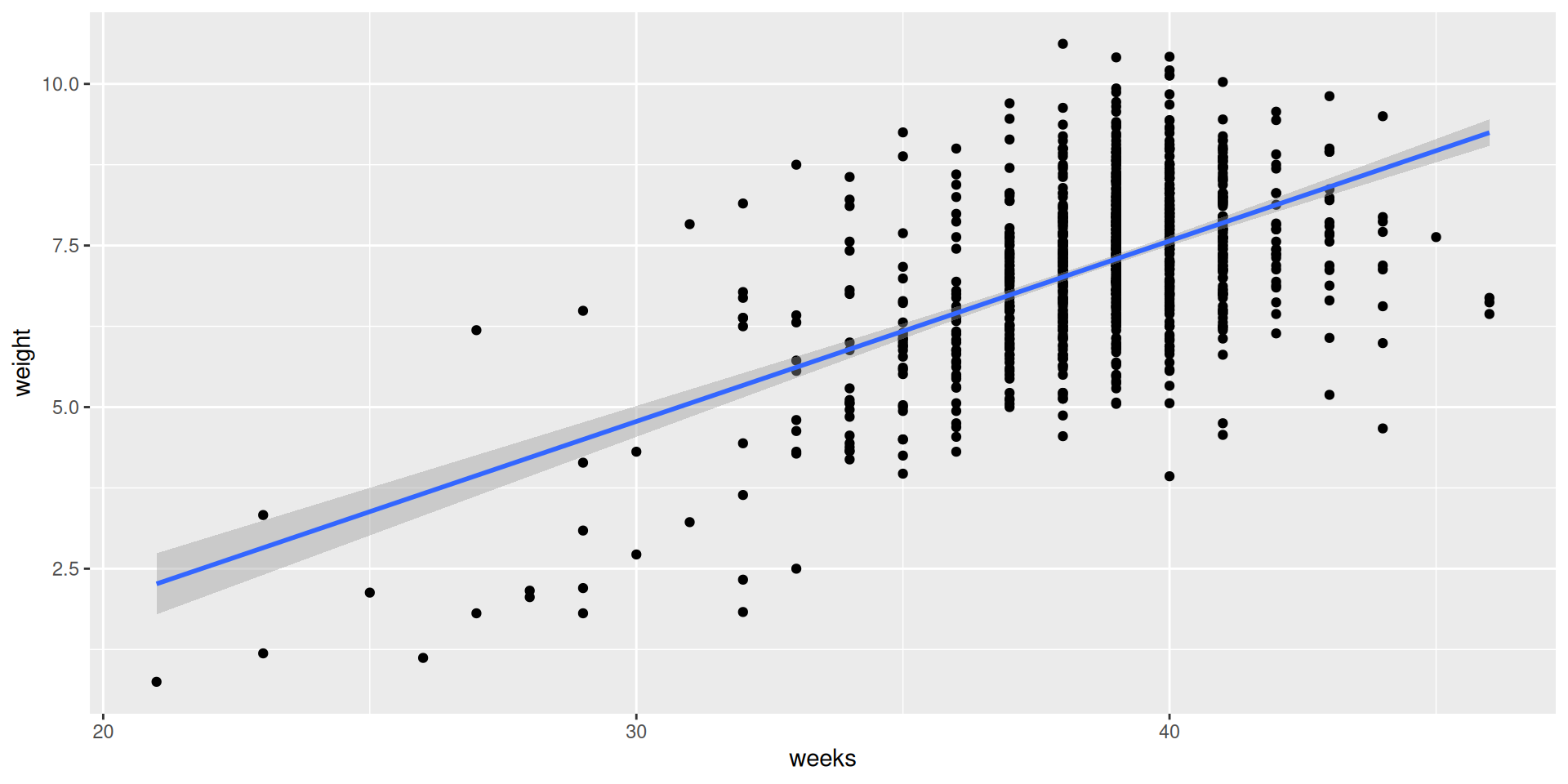
SLR model
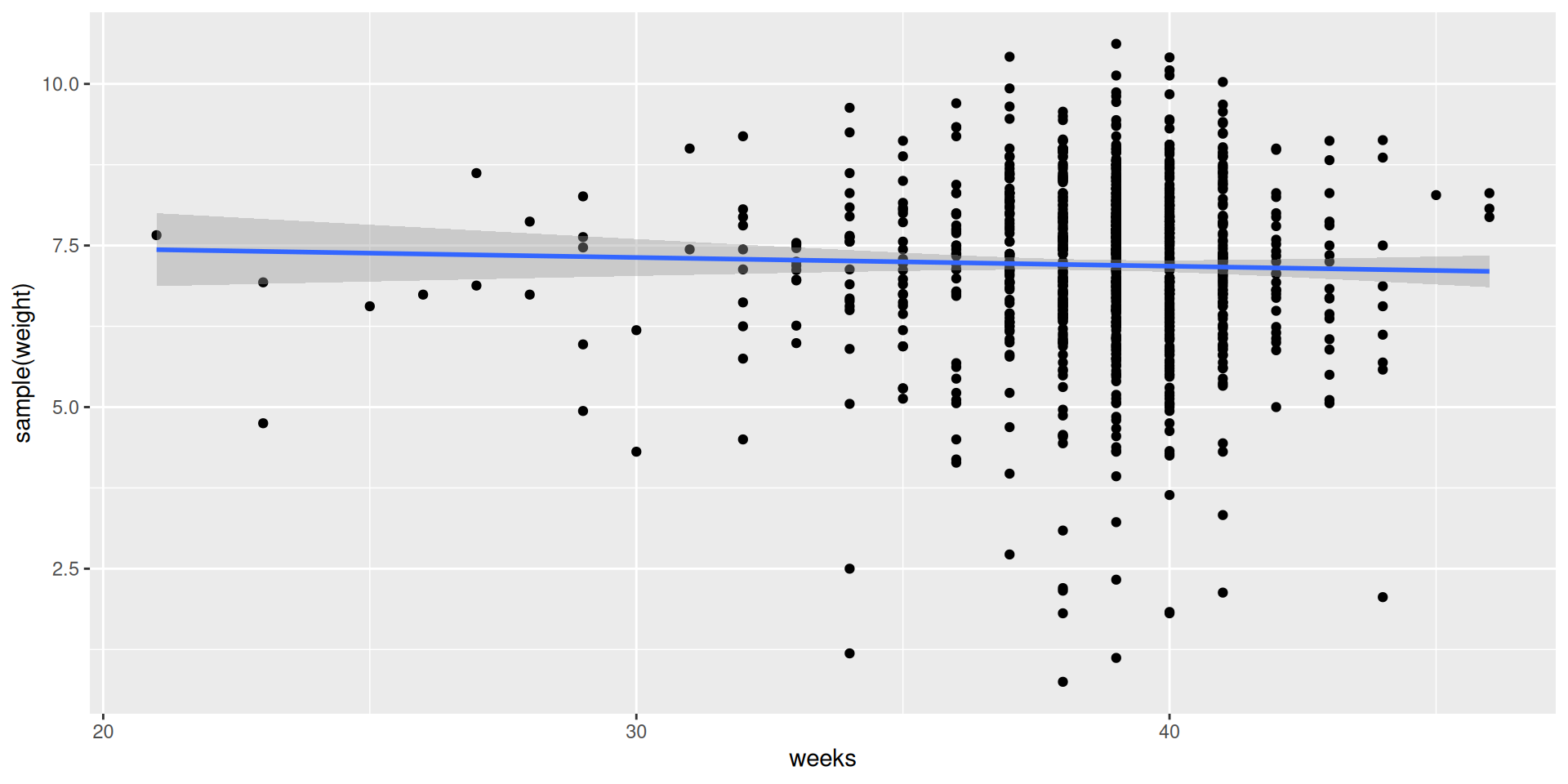
Simulate the null distribution
# A tibble: 1 × 1
      se
   <dbl>
1 0.0161Just one shuffled slope!
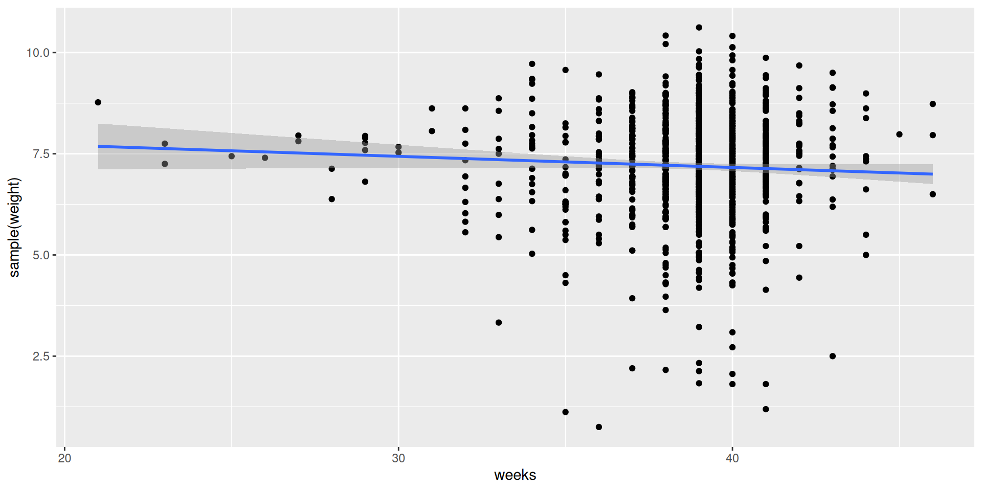
And another one…
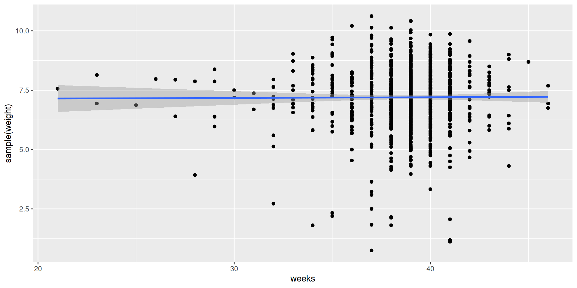
And one more…
Where is the test statistic?
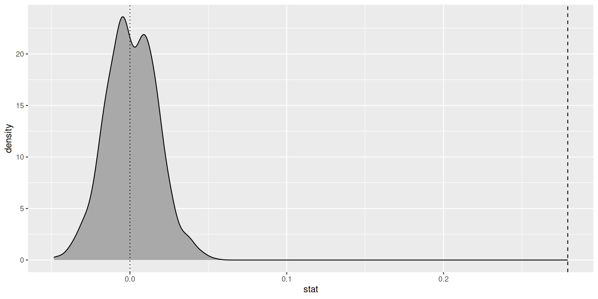
Decision
We reject the null hypothesis that the true slope coefficient \(\beta_1 = 0\)
Gestational length has a statistically significant positive association with birthweight
Each additional week that a baby remains in the womb is associated with an increase in the expected birthweight of about one quarter of a pound (about the weight of 🍔)
\(t\)-based approximation
\(t\)-test
Call:
lm(formula = weight ~ weeks, data = births14)

Residuals:
    Min      1Q  Median      3Q     Max
-4.0175 -0.7187  0.0190  0.6886  3.6078

Coefficients:
            Estimate Std. Error t value Pr(>|t|)
(Intercept) -3.59797    0.52273  -6.883 1.03e-11 ***
weeks        0.27922    0.01349  20.699  < 2e-16 ***
---
Signif. codes:  0 '***' 0.001 '**' 0.01 '*' 0.05 '.' 0.1 ' ' 1

Residual standard error: 1.094 on 998 degrees of freedom
Multiple R-squared:  0.3004,    Adjusted R-squared:  0.2997
F-statistic: 428.4 on 1 and 998 DF,  p-value: < 2.2e-16
Using broom
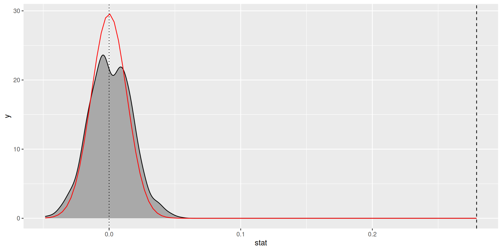
How good is the approximation?
Confidence intervals
Recall our bootstrap CI
Parametric confidence intervals are of the form: \[ \text{estimate} \pm \text{multiplier} \cdot \text{standard error} \]
\(t\)-confidence intervals for each coefficient have the form: \[ \hat{\beta_j} \pm \text{multiplier} \cdot \text{standard error}_{\hat{\beta}_j} \]
Computing confidence intervals
   lower_ci  upper_ci
1 0.2490562 0.3130666 2.5 % 97.5 %
(Intercept) -4.6237403 -2.572200
weeks 0.2527442 0.305686# A tibble: 2 × 7
term estimate std.error statistic p.value conf.low conf.high
<chr> <dbl> <dbl> <dbl> <dbl> <dbl> <dbl>
1 (Intercept) -3.60 0.523 -6.88 1.03e-11 -4.62 -2.57
2 weeks 0.279 0.0135 20.7 1.80e-79 0.253 0.306Diagnostics
Checking conditions
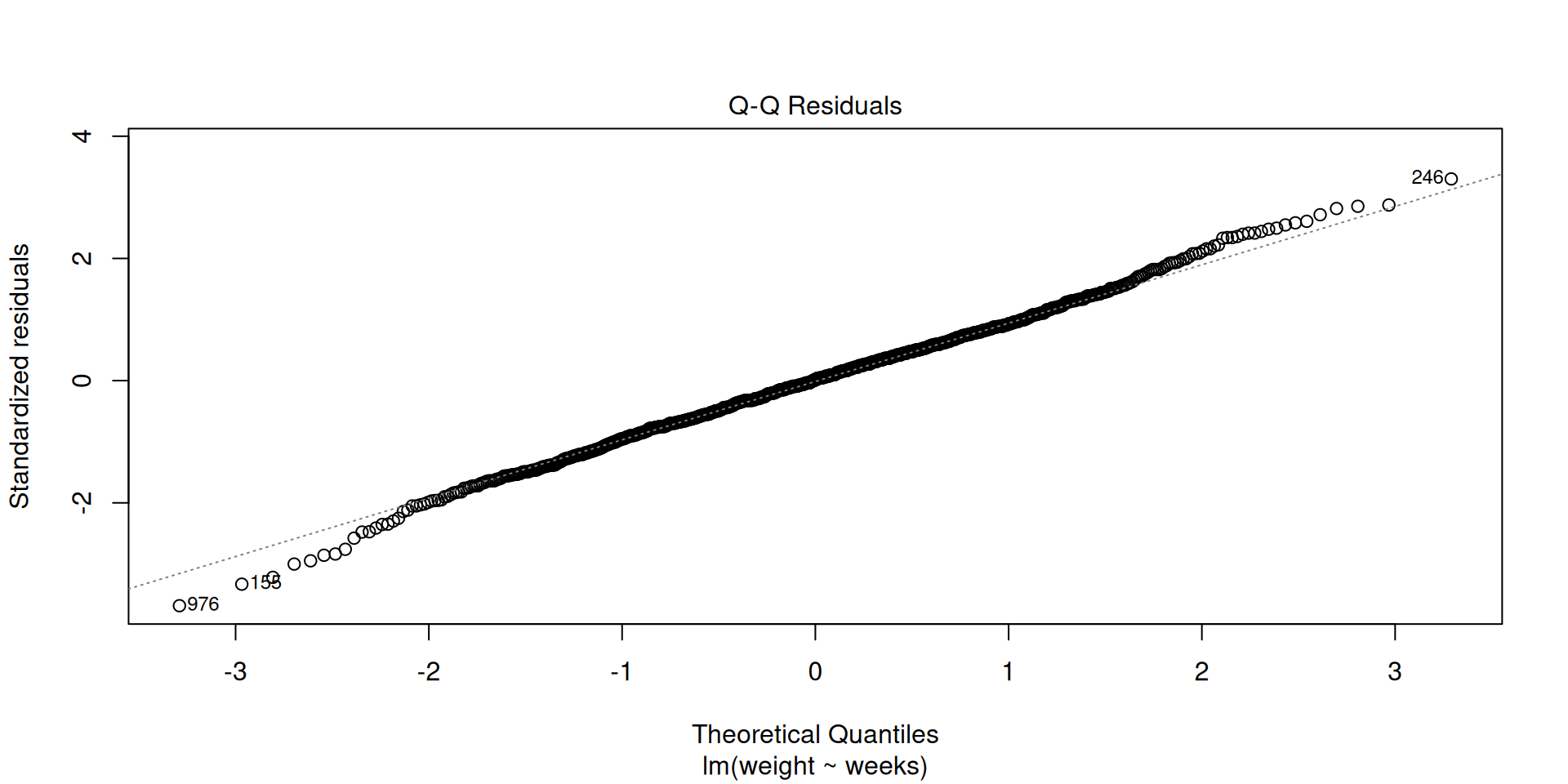
We assumed the slope coefficient followed a \(t\)-distribution
When we fit the regression model: \[ Y = \beta_0 + \beta_1 \cdot X + \epsilon \, , \]
We assume that \(\epsilon \sim N(0, \sigma)\), for some constant \(\sigma\)
L-I-N-E
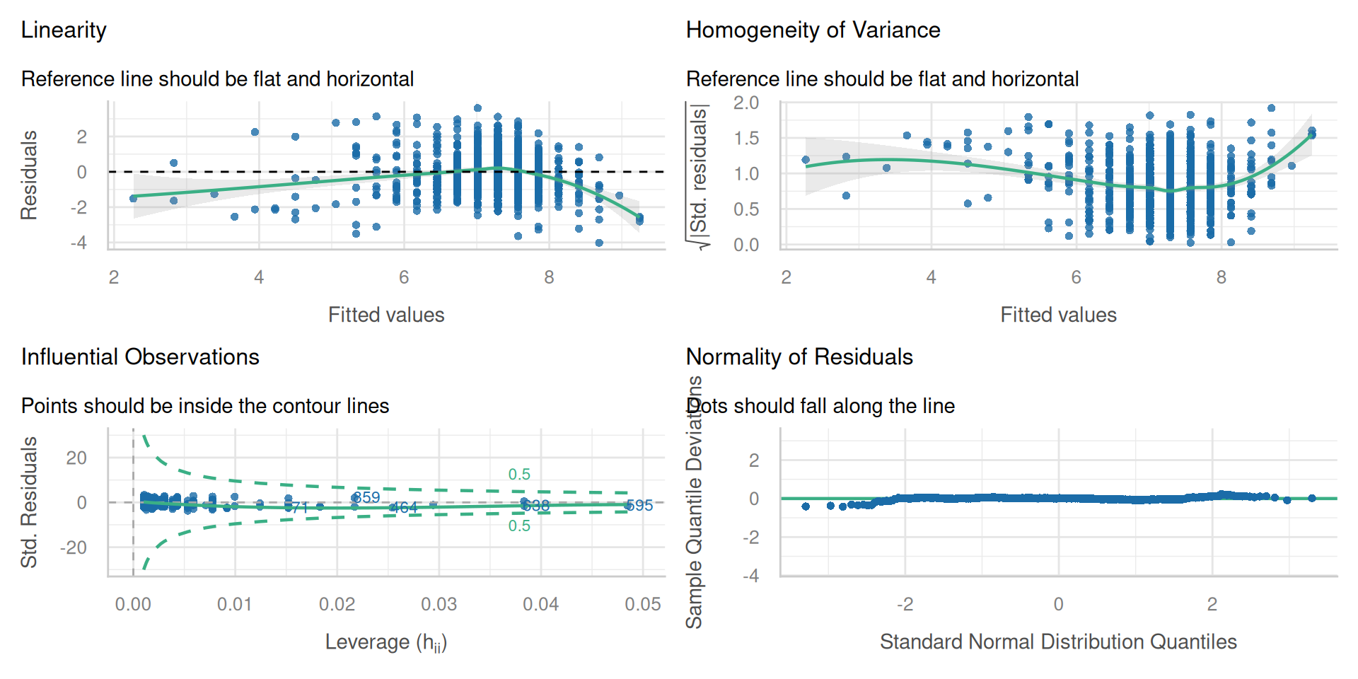
- Our inferences will only be valid if the following assumptions are reasonable:
- Linearity
- Independence (of residuals)
- Normality (of residuals)
- Equal Variance (of residuals)
Linearity (and independence)
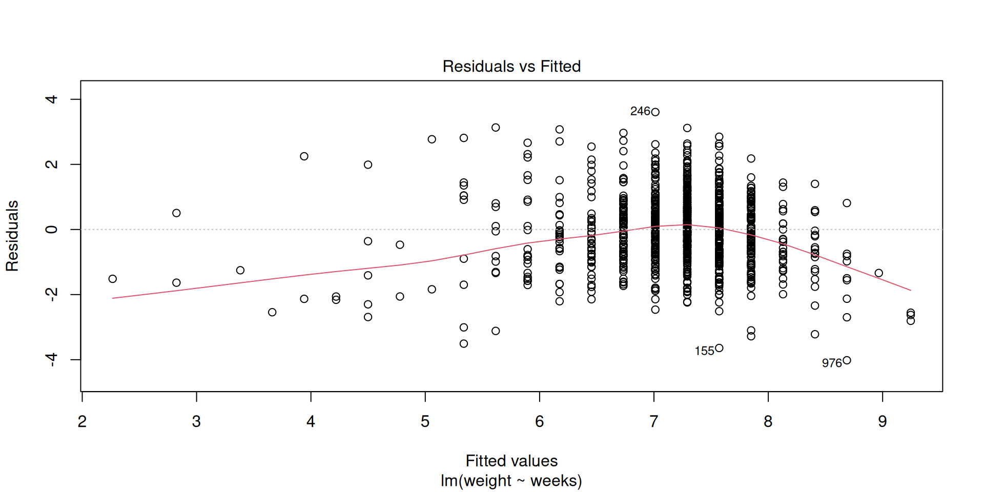
Normality of residuals
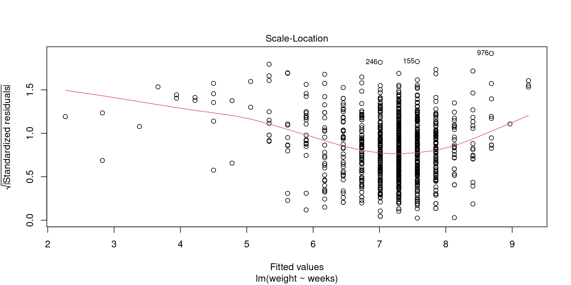
Equal variance
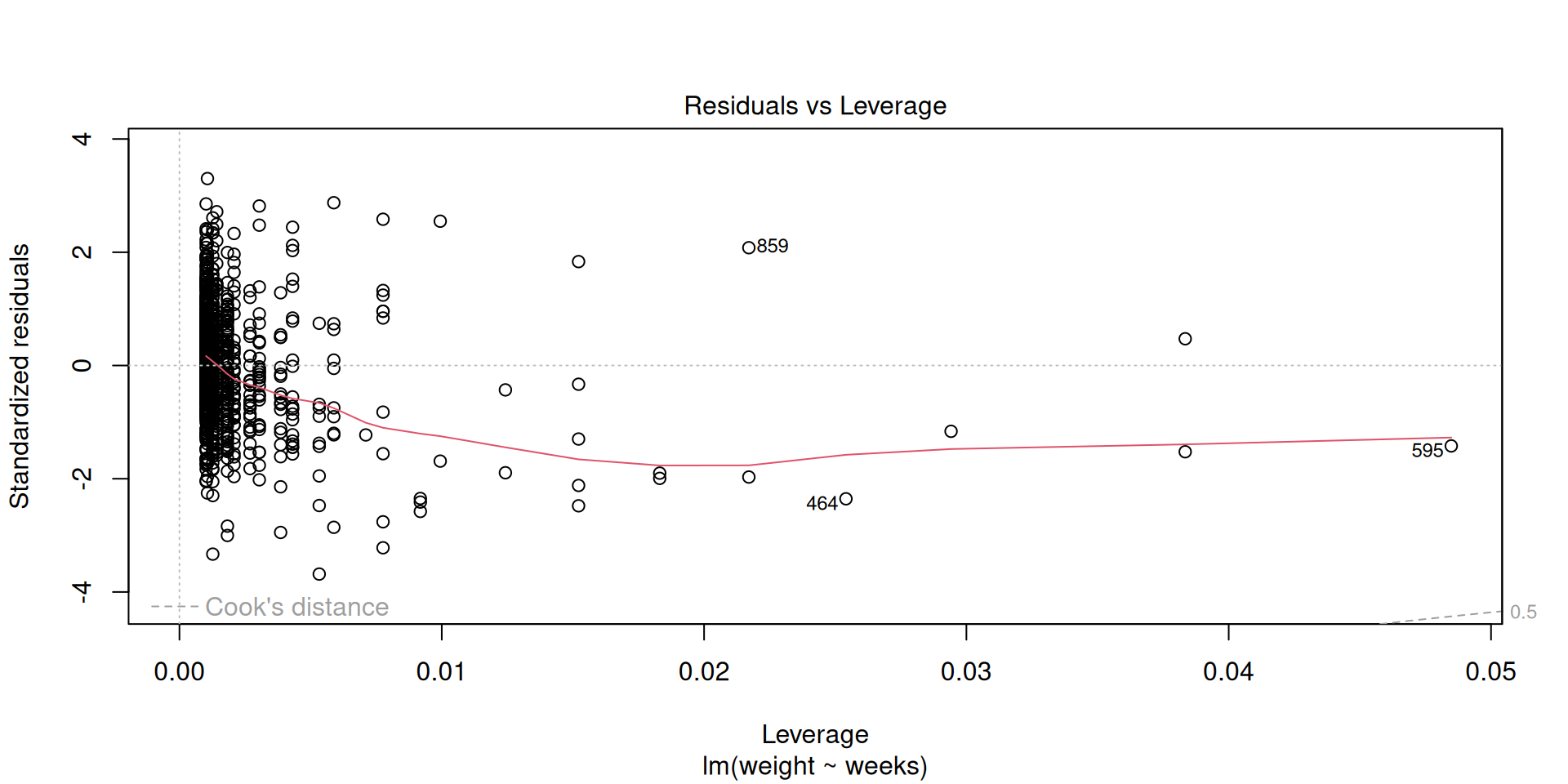
Influential points
Check all conditions
In-class micro-project
Teacher salaries
Recall the teacher salaries data set
openintro::teacherUse
yearsof experience as an explanatory variable fortotalsalaryFit, interpret, and assess the model