Diagnostic plots for seg_basket objects

Diagnostic plots for seg_basket objects

Usage

plot_best_chromosome(x)

plot_cpt_repeated(x, i = nrow(x$basket))

Arguments

x

A seg_basket() object

i

index of basket to show

Value

A ggplot2::ggplot() object

Details

seg_basket() objects contain baskets of candidate changepoint sets.

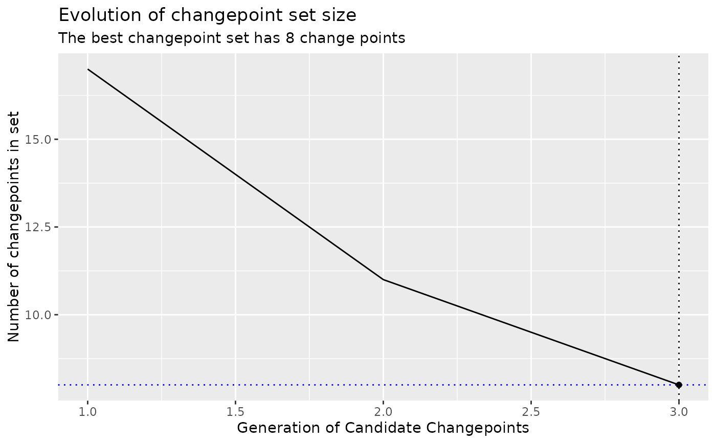
plot_best_chromosome() shows how the size of the candidate changepoint sets change across the generations of evolution.

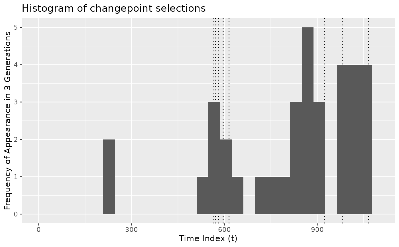
plot_cpt_repeated() shows how frequently individual observations appear in the best candidate changepoint sets in each generation.

Examples

# \donttest{
# Segment a time series using Coen's algorithm
x <- segment(DataCPSim, method = "coen", num_generations = 3)
#> 
  |                                                                  
  |                                                            |   0%
  |                                                                  
  |==============================                              |  50%
  |                                                                  
  |============================================================| 100%

# Plot the size of the sets during the evolution
x |>
  as.segmenter() |>
  plot_best_chromosome()

# }
# \donttest{
# Segment a time series using Coen's algorithm
x <- segment(DataCPSim, method = "coen", num_generations = 3)
#> 
  |                                                                  
  |                                                            |   0%
  |                                                                  
  |==============================                              |  50%
  |                                                                  
  |============================================================| 100%

# Plot overall frequency of appearance of changepoints
plot_cpt_repeated(x$segmenter)
#> `stat_bin()` using `bins = 30`. Pick better value `binwidth`.
#> Warning: Removed 2 rows containing missing values or values outside the scale range
#> (`geom_bar()`).


# Plot frequency of appearance only up to a specific generation
plot_cpt_repeated(x$segmenter, 5)
#> `stat_bin()` using `bins = 30`. Pick better value `binwidth`.
#> Warning: Removed 2 rows containing missing values or values outside the scale range
#> (`geom_bar()`).

# }