Climate data in tidychangepoint • tidychangepoint

The tidychangepoint package (Baumer and Suarez Sierra 2024) provides three climate-related time series.

library(tidychangepoint)

Central England Temperature

Shi et al. (2022) use changepoint detection algorithms to analyze a time series of annual temperature data from Central England. These data are available via CET from tidychangepoint.

These data go back to 1659, and a simple plot illustrates the increase in temperature in recent years.

plot(CET)

Shi et al. (2022) use a genetic algorithm to identify changepoints in this time series. The code below reproduces this analysis. Note that since the genetic algorithm is random, results vary. Shi, et al. used a maxiter value of 50,000 in order to obtain the results used in the paper. Here, we use a much lower value solely in the interest of computational speed. Note that this algorithm is fitting a “meanshift” model, which estimates the mean \(\mu_i\) for each of the regions defined by the changepoint set. The objective function employs the BIC penalty. One departure from Shi’s implementation is the use of the log_gabin_population() function to generate the first generation of 200 (i.e. popSize) possible changepoint sets. Each data point is chosen uniformly at random with probability equal to \(\ln{N}\), where \(N\) is the number of observations (362, in this case).

trend_wn <- CET |>
  segment(
    method = "ga", 
    model_fn = fit_meanshift_norm, 
    penalty_fn = BIC, 
    population = log_gabin_population(CET),
    popSize = 200, 
    maxiter = 50,
    run = 10
  )

## Seeding initial population with probability: 0.0162752602536624

Compare this with the changepoint set discovered by the algorithm:

changepoints(trend_wn)

##  x30  x41 x266 x331 
##   30   41  266  331

changepoints(trend_wn, use_labels = TRUE) |>
  as_year()

## [1] "1688" "1699" "1924" "1989"

The fitness() function returns a named vector with the value of the objective function from the discovered changepoint set.

fitness(trend_wn)

##      BIC 
## 653.2597

Information about the regions, including their means, are shown by the tidy() function.

tidy(trend_wn)

## # A tibble: 5 × 9
##   region    num_obs   min   max  mean    sd begin   end param_mu
##   <chr>       <int> <dbl> <dbl> <dbl> <dbl> <dbl> <dbl>    <dbl>
## 1 [0,30)         29  7.88 10.2   8.89 0.543     0    30     8.89
## 2 [30,41)        11  7.29  8.94  8.08 0.496    30    41     8.08
## 3 [41,266)      225  6.86 10.5   9.17 0.593    41   266     9.17
## 4 [266,331)      65  8.52 10.6   9.52 0.437   266   331     9.52
## 5 [331,362]      32  8.86 11.0  10.3  0.497   331   362    10.3

By default, glance() returns a summary of the segmenter that produced the discovered changepoint set. This includes the fitness, the elapsed time, and the parameters used by the segmenter.

glance(trend_wn)

## # A tibble: 1 × 8
##   pkg   version    algorithm seg_params model_name criteria fitness elapsed_time
##   <chr> <pckg_vrs> <chr>     <list>     <chr>      <chr>      <dbl> <drtn>      
## 1 GA    3.2.4      Genetic   <list [1]> meanshift… BIC         653. 9.822 secs

However, we can also run glance() on the model resulting from the discovered changepoint set. This provides information about the model and its fit, including the values of various alternative model fitting metrics.

It is important to note that only one of these metrics (in this case, BIC) is actually the one used by the segmenter!

trend_wn |>
  as.model() |>
  glance()

## # A tibble: 1 × 11
##   pkg     version algorithm params num_cpts  rmse logLik   AIC   BIC  MBIC   MDL
##   <chr>   <pckg_> <chr>     <list>    <int> <dbl>  <dbl> <dbl> <dbl> <dbl> <dbl>
## 1 tidych… 0.0.1   meanshif… <dbl>         4 0.550  -297.  614.  653.  654.  664.

The plot() function returns an informative plot of the original time series, with the changepoint set and the corresponding regions demarcated.

plot(trend_wn, use_time_index = TRUE)

## Scale for x is already present.
## Adding another scale for x, which will replace the existing scale.

Comparison to reported values

The changepoint set reported by Shi et al. (2022) is \(\{1700, 1739, 1988\}\). For that configuration with the trendshift model with white noise errors, Table 2 of Shi et al. (2022) reports model variance \(\hat{\sigma}^2\) of 0.291, a log-likelihood of -290.02, BIC of 650.74, and MDL of 653.07.

Fitting the trendshift model with white noise errors and running the glance() function reveals an exact match to the reported figures.

target_cpts <- c(1700, 1739, 1988)
ids <- time2tau(target_cpts, as_year(time(CET)))
CET |>
  fit_trendshift(tau = ids) |>
  glance()

## # A tibble: 1 × 11
##   pkg     version algorithm params num_cpts  rmse logLik   AIC   BIC  MBIC   MDL
##   <chr>   <pckg_> <chr>     <list>    <int> <dbl>  <dbl> <dbl> <dbl> <dbl> <dbl>
## 1 tidych… 0.0.1   trendshi… <dbl>         3 0.539  -290.  604.  651.  626.  653.

Modifying the model to incorporate AR(1) lagged errors also matches the figures from Table 2.

CET |>
  fit_trendshift_ar1(tau = ids) |>
  glance()

## # A tibble: 1 × 11
##   pkg     version algorithm params num_cpts  rmse logLik   AIC   BIC  MBIC   MDL
##   <chr>   <pckg_> <chr>     <list>    <int> <dbl>  <dbl> <dbl> <dbl> <dbl> <dbl>
## 1 tidych… 0.0.1   trendshi… <dbl>         3 0.538  -289.  603.  654.  623.  656.

Bogotá particulate matter

The bogota_pm data set contains daily measurement on particulate matter in Bogotá, Colombia over the three-year period from 2018–2020.

plot(bogota_pm)

Here, we use the genetic algorithm from Taimal, Suárez-Sierra, and Rivera (2023) to identify changepoint sets. Note that the model being fit here is the NHPP model, along with the BMDL penalty function.

bog_cpt <- bogota_pm |>
  segment(
    method = "ga-coen",
    maxiter = 50,
    run = 10
  )

## Seeding initial population with probability: 0.0145985401459854

glance(bog_cpt)

## # A tibble: 1 × 8
##   pkg   version    algorithm seg_params model_name criteria fitness elapsed_time
##   <chr> <pckg_vrs> <chr>     <list>     <chr>      <chr>      <dbl> <drtn>      
## 1 GA    3.2.4      Genetic   <list [1]> nhpp       BMDL       1987. 33.462 secs

plot(bog_cpt, use_time_index = TRUE)

## Scale for x is already present.
## Adding another scale for x, which will replace the existing scale.

We compare the quality of the fit of the NHPP model using diagnose().

bog_cpt |>
  as.model() |>
  diagnose()

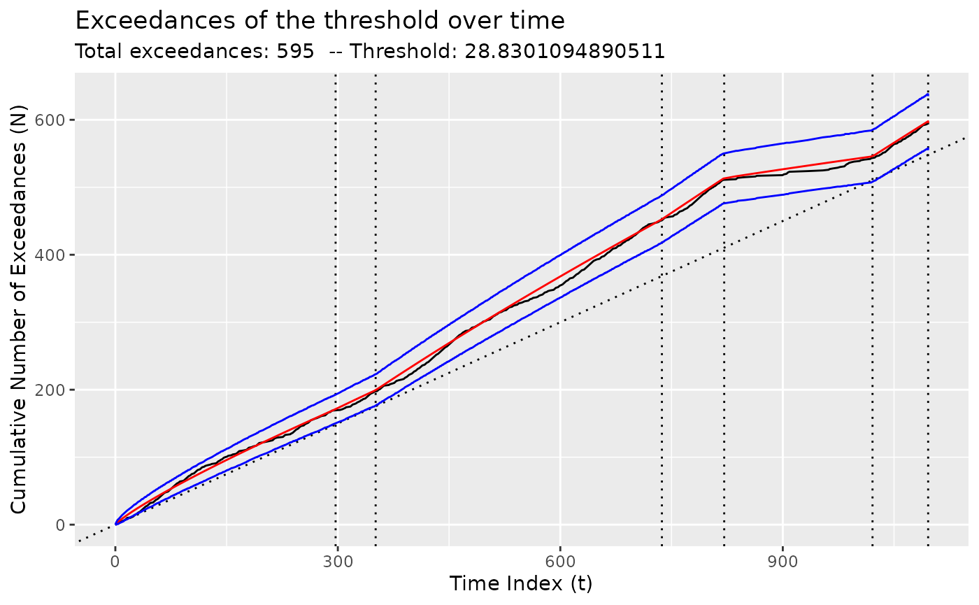
Medellín rainfall

The times series mde_rain_monthly contains monthly precipitation readings from locations in and around the city of Medellín, Colombia.

plot(mde_rain_monthly)

Here, we fit the deterministic PELT algorithm (Killick and Eckley 2014).

mde_cpt <- segment(mde_rain_monthly, method = "pelt")

plot(mde_cpt, use_time_index = TRUE)

## Scale for x is already present.
## Adding another scale for x, which will replace the existing scale.

References

Baumer, Benjamin S., and Biviana Marcela Suarez Sierra. 2024. “Tidychangepoint: A Unified Framework for Analyzing Changepoint Detection in Univariate Time Series.” https://beanumber.github.io/changepoint-paper/.

Killick, Rebecca, and Idris A. Eckley. 2014. “changepoint: An R Package for Changepoint Analysis.” Journal of Statistical Software 58 (3): 1–19. 10.18637/jss.v058.i03.

Shi, Xueheng, Claudie Beaulieu, Rebecca Killick, and Robert Lund. 2022. “Changepoint Detection: An Analysis of the Central England Temperature Series.” Journal of Climate 35 (19): 6329–42. https://doi.org/10.1175/JCLI-D-21-0489.1.

Taimal, Carlos A, Biviana Marcela Suárez-Sierra, and Juan Carlos Rivera. 2023. “An Exploration of Genetic Algorithms Operators for the Detection of Multiple Change-Points of Exceedances Using Non-Homogeneous Poisson Processes and Bayesian Methods.” In Colombian Conference on Computing, 230–58. Springer. https://doi.org/10.1007/978-3-031-47372-2_20.