Objects exported from other packages
reexports.RdThese objects are imported from other packages. Follow the links below to see their documentation.
Usage
# S3 method for class 'mod_cpt'
as.ts(x, ...)

# S3 method for class 'mod_cpt'
nobs(object, ...)

# S3 method for class 'mod_cpt'
logLik(object, ...)

# S3 method for class 'mod_cpt'
fitted(object, ...)

# S3 method for class 'mod_cpt'
residuals(object, ...)

# S3 method for class 'mod_cpt'
coef(object, ...)

# S3 method for class 'mod_cpt'
augment(x, ...)

# S3 method for class 'mod_cpt'
tidy(x, ...)

# S3 method for class 'mod_cpt'
glance(x, ...)

# S3 method for class 'mod_cpt'
plot(x, ...)

# S3 method for class 'mod_cpt'
print(x, ...)

# S3 method for class 'mod_cpt'
summary(object, ...)

# S3 method for class 'seg_basket'
as.ts(x, ...)

# S3 method for class 'seg_basket'
plot(x, ...)

# S3 method for class 'seg_cpt'
as.ts(x, ...)

# S3 method for class 'seg_cpt'
glance(x, ...)

# S3 method for class 'seg_cpt'
nobs(object, ...)

# S3 method for class 'seg_cpt'
print(x, ...)

# S3 method for class 'seg_cpt'
summary(object, ...)

# S3 method for class 'tidycpt'
as.ts(x, ...)

# S3 method for class 'tidycpt'
augment(x, ...)

# S3 method for class 'tidycpt'
tidy(x, ...)

# S3 method for class 'tidycpt'
glance(x, ...)

# S3 method for class 'tidycpt'
plot(x, use_time_index = FALSE, ylab = NULL, ...)

# S3 method for class 'tidycpt'
print(x, ...)

# S3 method for class 'tidycpt'
summary(object, ...)

# S3 method for class 'meanshift_lnorm'
logLik(object, ...)

# S3 method for class 'nhpp'
logLik(object, ...)

# S3 method for class 'nhpp'
glance(x, ...)

# S3 method for class 'ga'
as.ts(x, ...)

# S3 method for class 'ga'
nobs(object, ...)

# S3 method for class 'cpt'
as.ts(x, ...)

# S3 method for class 'cpt'
logLik(object, ...)

# S3 method for class 'cpt'
nobs(object, ...)

# S3 method for class 'cptga'
as.ts(x, ...)

# S3 method for class 'cptga'
nobs(object, ...)

# S3 method for class 'segmented'
as.ts(x, ...)

# S3 method for class 'stepmented'
as.ts(x, ...)

# S3 method for class 'breakpointsfull'
as.ts(x, ...)

# S3 method for class 'breakpointsfull'
nobs(object, ...)

# S3 method for class 'wbs'
as.ts(x, ...)

# S3 method for class 'wbs'
nobs(object, ...)Examples
# Plot a meanshift model fit
plot(fit_meanshift_norm(CET, tau = 330))
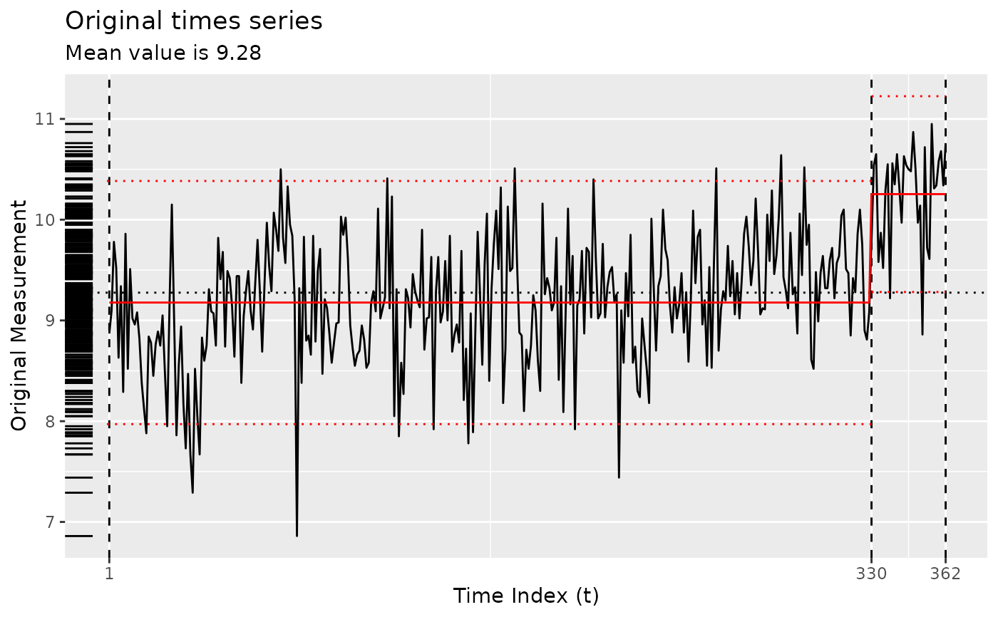 plot(fit_meanshift_norm(CET, tau = 330), plot.title.position = "plot")
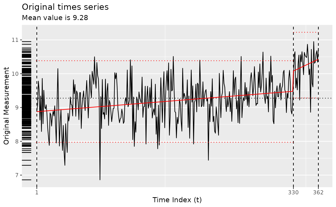 #' # Plot a trendshift model fit
plot(fit_trendshift(CET, tau = 330))
#' # Plot a trendshift model fit
plot(fit_trendshift(CET, tau = 330))
 #' # Plot a quadratic polynomial model fit
plot(fit_lmshift(CET, tau = 330, deg_poly = 2))
#' # Plot a quadratic polynomial model fit
plot(fit_lmshift(CET, tau = 330, deg_poly = 2))
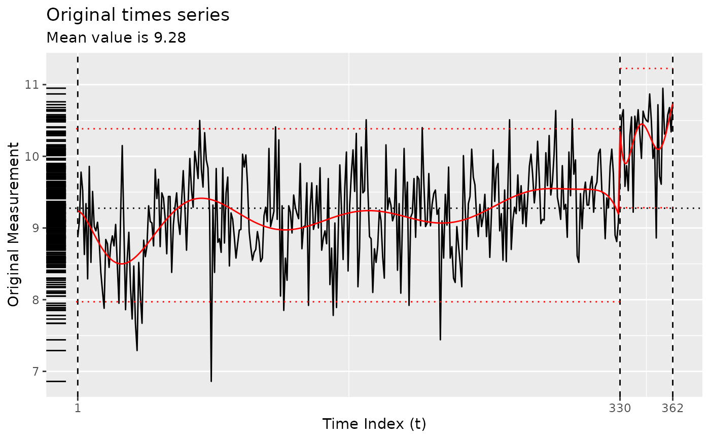 #' # Plot a 4th degree polynomial model fit
plot(fit_lmshift(CET, tau = 330, deg_poly = 10))
#' # Plot a 4th degree polynomial model fit
plot(fit_lmshift(CET, tau = 330, deg_poly = 10))
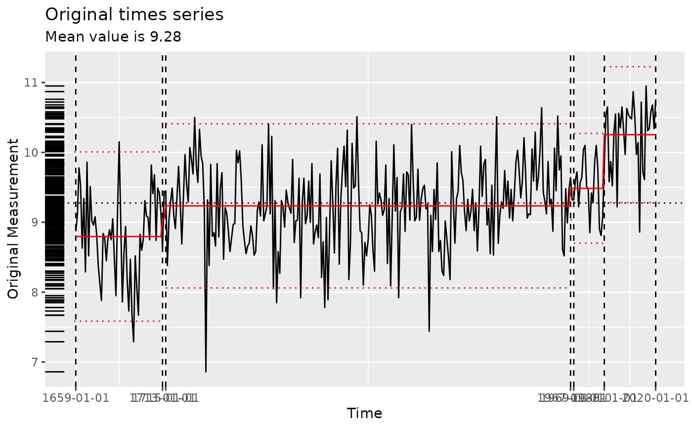
 # Plot a segmented time series
plot(segment(CET, method = "pelt"))
# Plot a segmented time series
plot(segment(CET, method = "pelt"))
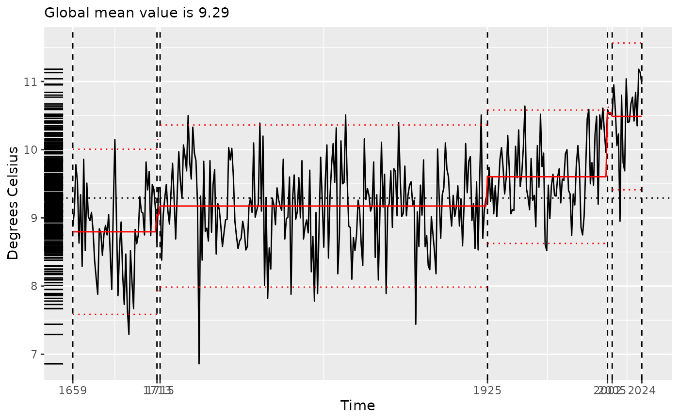
 # Plot a segmented time series and show the time labels on the x-axis
plot(segment(CET, method = "pelt"), use_time_index = TRUE)
#> Scale for x is already present.
#> Adding another scale for x, which will replace the existing scale.
# Plot a segmented time series and show the time labels on the x-axis
plot(segment(CET, method = "pelt"), use_time_index = TRUE)
#> Scale for x is already present.
#> Adding another scale for x, which will replace the existing scale.
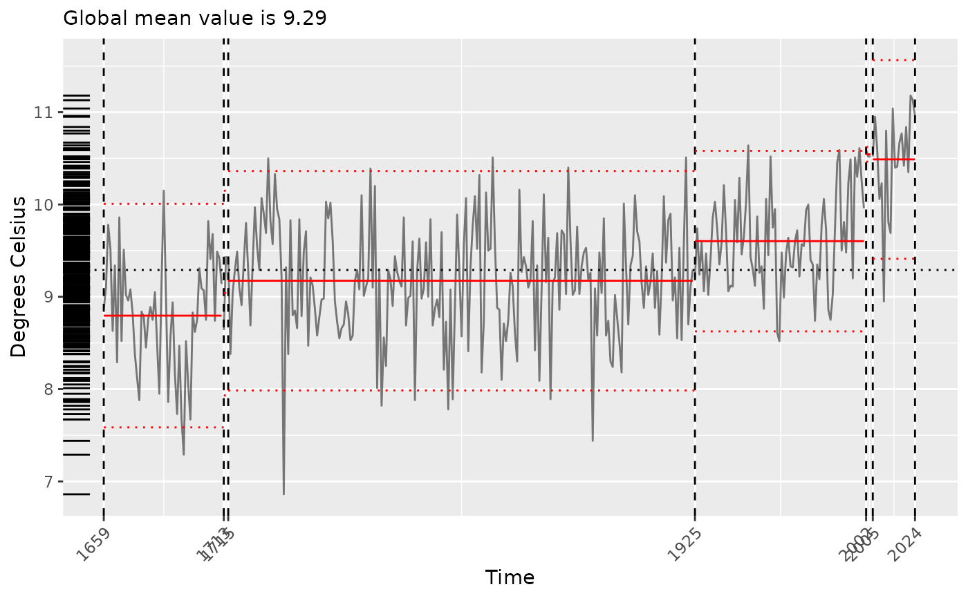
 # Label the y-axis correctly
segment(CET, method = "pelt") |>
plot(use_time_index = TRUE, ylab = "Degrees Celsius")
#> Scale for x is already present.
#> Adding another scale for x, which will replace the existing scale.
# Label the y-axis correctly
segment(CET, method = "pelt") |>
plot(use_time_index = TRUE, ylab = "Degrees Celsius")
#> Scale for x is already present.
#> Adding another scale for x, which will replace the existing scale.
 # Summarize a tidycpt object
summary(segment(CET, method = "pelt"))
#>
#> ── Summary of tidycpt object ───────────────────────────────────────────────────
#> → y: Contains 366 observations, ranging from 6.86 to 11.18 .
#> ℹ Segmenter (class cpt )
#> → A: Used the PELT algorithm from the changepoint package.
#> → τ: Found 5 changepoint(s).
#> → f: Reported a fitness value of Inf using the MBIC penalty.
#> ℹ Model
#> → M: Fit the meanvar model.
#> → θ: Estimated 2 parameter(s), for each of 6 region(s).
summary(segment(DataCPSim, method = "pelt"))
#>
#> ── Summary of tidycpt object ───────────────────────────────────────────────────
#> → y: Contains 1096 observations, ranging from 13.67 to 298.98 .
#> ℹ Segmenter (class cpt )
#> → A: Used the PELT algorithm from the changepoint package.
#> → τ: Found 3 changepoint(s).
#> → f: Reported a fitness value of 9.40 k using the MBIC penalty.
#> ℹ Model
#> → M: Fit the meanvar model.
#> → θ: Estimated 2 parameter(s), for each of 4 region(s).
# Summarize a tidycpt object
summary(segment(CET, method = "pelt"))
#>
#> ── Summary of tidycpt object ───────────────────────────────────────────────────
#> → y: Contains 366 observations, ranging from 6.86 to 11.18 .
#> ℹ Segmenter (class cpt )
#> → A: Used the PELT algorithm from the changepoint package.
#> → τ: Found 5 changepoint(s).
#> → f: Reported a fitness value of Inf using the MBIC penalty.
#> ℹ Model
#> → M: Fit the meanvar model.
#> → θ: Estimated 2 parameter(s), for each of 6 region(s).
summary(segment(DataCPSim, method = "pelt"))
#>
#> ── Summary of tidycpt object ───────────────────────────────────────────────────
#> → y: Contains 1096 observations, ranging from 13.67 to 298.98 .
#> ℹ Segmenter (class cpt )
#> → A: Used the PELT algorithm from the changepoint package.
#> → τ: Found 3 changepoint(s).
#> → f: Reported a fitness value of 9.40 k using the MBIC penalty.
#> ℹ Model
#> → M: Fit the meanvar model.
#> → θ: Estimated 2 parameter(s), for each of 4 region(s).