Segment a time series using a genetic algorithm

Segmenting functions for various genetic algorithms

Usage

segment_ga(
  x,
  model_fn = fit_meanshift_norm,
  penalty_fn = BIC,
  model_fn_args = list(),
  ...
)

segment_ga_shi(x, ...)

segment_ga_coen(x, ...)

segment_ga_random(x, ...)

Arguments

x: A time series
model_fn: A character or name coercible into a fun_cpt function. See, for example, fit_meanshift_norm().
penalty_fn: A function that evaluates the changepoint set returned by model_fn. We provide AIC(), BIC(), MBIC(), MDL(), and BMDL().
model_fn_args: A list() of parameters passed to model_fn
...: arguments passed to GA::ga()

Value

A tidyga object. This is just a GA::ga() object with an additional slot for data (the original time series) and model_fn_args (captures the model_fn and penalty_fn arguments).

Details

segment_ga() uses the genetic algorithm in GA::ga() to "evolve" a random set of candidate changepoint sets, using the penalized objective function specified by penalty_fn. By default, the normal meanshift model is fit (see fit_meanshift_norm()) and the BIC penalty is applied.

segment_ga_shi(): Shi's algorithm is the algorithm used in doi:10.1175/JCLI-D-21-0489.1 . Note that in order to achieve the reported results you have to run the algorithm for a really long time. Pass the values maxiter = 50000 and run = 10000 to GA::ga() using the dots.

segment_ga_coen(): Coen's algorithm is the one used in doi:10.1007/978-3-031-47372-2_20 . Note that the speed of the algorithm is highly sensitive to the size of the changepoint sets under consideration, with large changepoint sets being slow. Consider setting the population argument to GA::ga() to improve performance. Coen's algorithm uses the build_gabin_population() function for this purpose by default.

segment_ga_random(): Randomly select candidate changepoint sets. This is implemented as a genetic algorithm with only one generation (i.e., maxiter = 1). Note that this function uses log_gabin_population() by default.

References

Shi, et al. (2022, doi:10.1175/JCLI-D-21-0489.1 )

Taimal, et al. (2023, doi:10.1007/978-3-031-47372-2_20 )

Examples

# Segment a time series using a genetic algorithm
res <- segment_ga(CET, maxiter = 5)
summary(res)
#> ── Genetic Algorithm ─────────────────── 
#> 
#> GA settings: 
#> Type                  =  binary 
#> Population size       =  50 
#> Number of generations =  5 
#> Elitism               =  2 
#> Crossover probability =  0.8 
#> Mutation probability  =  0.1 
#> 
#> GA results: 
#> Iterations             = 5 
#> Fitness function value = -2206.599 
#> Solution = 
#>      x1 x2 x3 x4 x5 x6 x7 x8 x9 x10  ...  x361 x362
#> [1,]  0  1  1  0  0  1  1  1  0   0          0    0
str(res)
#> Formal class 'tidyga' [package "tidychangepoint"] with 23 slots
#>   ..@ data         : Time-Series [1:362] from 1 to 362: 8.87 9.1 9.78 9.52 8.63 9.34 8.29 9.86 8.52 9.51 ...
#>   ..@ model_fn_args:List of 2
#>   .. ..$ model_fn  : chr "meanshift_norm"
#>   .. ..$ penalty_fn: chr "BIC"
#>   ..@ call         : language GA::ga(type = "binary", fitness = obj_fun, nBits = n, maxiter = 5)
#>   ..@ type         : chr "binary"
#>   ..@ lower        : logi NA
#>   ..@ upper        : logi NA
#>   ..@ nBits        : int 362
#>   ..@ names        : chr [1:362] "x1" "x2" "x3" "x4" ...
#>   ..@ popSize      : num 50
#>   ..@ iter         : int 5
#>   ..@ run          : int 2
#>   ..@ maxiter      : num 5
#>   ..@ suggestions  : logi[0 , 1:362] 
#>   ..@ population   : num [1:50, 1:362] 0 1 1 0 1 1 1 0 0 1 ...
#>   ..@ elitism      : int 2
#>   ..@ pcrossover   : num 0.8
#>   ..@ pmutation    : num 0.1
#>   ..@ optim        : logi FALSE
#>   ..@ fitness      : num [1:50] -2274 -Inf -Inf -2207 -Inf ...
#>   ..@ summary      : num [1:5, 1:6] -2302 -2284 -2274 -2207 -2207 ...
#>   .. ..- attr(*, "dimnames")=List of 2
#>   .. .. ..$ : NULL
#>   .. .. ..$ : chr [1:6] "max" "mean" "q3" "median" ...
#>   ..@ bestSol      : list()
#>   ..@ fitnessValue : num -2207
#>   ..@ solution     : num [1, 1:362] 0 1 1 0 0 1 1 1 0 0 ...
#>   .. ..- attr(*, "dimnames")=List of 2
#>   .. .. ..$ : NULL
#>   .. .. ..$ : chr [1:362] "x1" "x2" "x3" "x4" ...
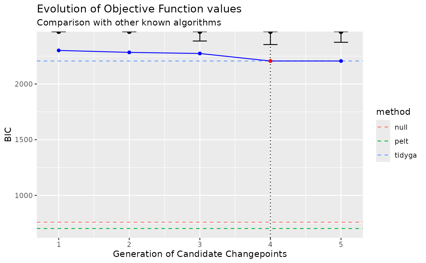
plot(res)


# \donttest{
# Segment a time series using Shi's algorithm
x <- segment(CET, method = "ga-shi", maxiter = 5)
str(x)
#> List of 4
#>  $ segmenter   :Formal class 'tidyga' [package "tidychangepoint"] with 23 slots
#>   .. ..@ data         : Time-Series [1:362] from 1 to 362: 8.87 9.1 9.78 9.52 8.63 9.34 8.29 9.86 8.52 9.51 ...
#>   .. ..@ model_fn_args:List of 2
#>   .. .. ..$ model_fn  : chr "meanshift_norm_ar1"
#>   .. .. ..$ penalty_fn: chr "BIC"
#>   .. ..@ call         : language GA::ga(type = "binary", fitness = obj_fun, nBits = n, popSize = 200, maxiter = 5)
#>   .. ..@ type         : chr "binary"
#>   .. ..@ lower        : logi NA
#>   .. ..@ upper        : logi NA
#>   .. ..@ nBits        : int 362
#>   .. ..@ names        : chr [1:362] "x1" "x2" "x3" "x4" ...
#>   .. ..@ popSize      : num 200
#>   .. ..@ iter         : int 5
#>   .. ..@ run          : int 3
#>   .. ..@ maxiter      : num 5
#>   .. ..@ suggestions  : logi[0 , 1:362] 
#>   .. ..@ population   : num [1:200, 1:362] 0 0 0 1 0 1 1 1 0 0 ...
#>   .. ..@ elitism      : int 10
#>   .. ..@ pcrossover   : num 0.8
#>   .. ..@ pmutation    : num 0.1
#>   .. ..@ optim        : logi FALSE
#>   .. ..@ fitness      : num [1:200] -Inf -Inf -2258 -Inf -2202 ...
#>   .. ..@ summary      : num [1:5, 1:6] -2225 -2225 -2202 -2202 -2202 ...
#>   .. .. ..- attr(*, "dimnames")=List of 2
#>   .. .. .. ..$ : NULL
#>   .. .. .. ..$ : chr [1:6] "max" "mean" "q3" "median" ...
#>   .. ..@ bestSol      : list()
#>   .. ..@ fitnessValue : num -2202
#>   .. ..@ solution     : num [1, 1:362] 0 1 0 1 1 0 1 1 0 0 ...
#>   .. .. ..- attr(*, "dimnames")=List of 2
#>   .. .. .. ..$ : NULL
#>   .. .. .. ..$ : chr [1:362] "x1" "x2" "x3" "x4" ...
#>  $ model       :List of 7
#>   ..$ data         : Time-Series [1:362] from 1 to 362: 8.87 9.1 9.78 9.52 8.63 9.34 8.29 9.86 8.52 9.51 ...
#>   ..$ tau          : int [1:159] 2 4 5 7 8 13 15 16 20 23 ...
#>   ..$ region_params: tibble [160 × 2] (S3: tbl_df/tbl/data.frame)
#>   .. ..$ region  : chr [1:160] "[0,2)" "[2,4)" "[4,5)" "[5,7)" ...
#>   .. ..$ param_mu: num [1:160] 8.87 9.44 9.52 8.98 8.29 ...
#>   ..$ model_params : Named num [1:2] 0.139 -0.309
#>   .. ..- attr(*, "names")= chr [1:2] "sigma_hatsq" "phi_hat"
#>   ..$ fitted_values: num [1:362] 8.87 9.44 9.55 9.41 8.98 ...
#>   ..$ model_name   : chr "meanshift_norm_ar1"
#>   ..$ durbin_watson: num 2.62
#>   ..- attr(*, "class")= chr "mod_cpt"
#>  $ elapsed_time: 'difftime' num 0.886864423751831
#>   ..- attr(*, "units")= chr "secs"
#>  $ time_index  : Date[1:362], format: "1659-01-01" "1660-01-01" ...
#>  - attr(*, "class")= chr "tidycpt"

# Segment a time series using Coen's algorithm
y <- segment(CET, method = "ga-coen", maxiter = 5)
#> Seeding initial population with probability: 0.0359116022099447
changepoints(y)
#>  x8 x16 x37 x48 
#>   8  16  37  48 

# Segment a time series using Coen's algorithm and an arbitrary threshold
z <- segment(CET, method = "ga-coen", maxiter = 5, 
             model_fn_args = list(threshold = 2))
#> Seeding initial population with probability: 0.0331491712707182
changepoints(z)
#>  x23 x136 
#>   23  136 
# }
if (FALSE) { # \dontrun{
# This will take a really long time!
x <- segment(CET, method = "ga-shi", maxiter = 500, run = 100)
changepoints(x)

# This will also take a really long time!
y <- segment(CET, method = "ga", model_fn = fit_lmshift, penalty_fn = BIC, 
  popSize = 200, maxiter = 5000, run = 1000, 
  model_fn_args = list(trends = TRUE), 
  population = build_gabin_population(CET)
)
} # }

if (FALSE) { # \dontrun{
x <- segment(method = "ga-coen", maxiter = 50)
} # }

x <- segment(CET, method = "random")
#> Seeding initial population with probability: 0.0162752602536624