

1 The Baseball Datasets
1.1 Introduction
Baseball’s marriage with numbers goes back to the origins of the sport. When the first box scores and the first stats appeared in newspapers in the 1840s, the pioneers of the game had not yet decided the ultimate distance between the pitcher’s rubber and home plate, nor the number of balls needed to be awarded a base.
This chapter introduces four rich sources of freely available baseball data: the Lahman database, Retrosheet, PITCHf/x, and Statcast via Baseball Savant. Baseball records from these sources have a growing level of detail, from seasonal stats available since the 1871 season, to box score data for individual games, to play-by-play accounts covering most games since 1913, to extremely detailed pitch-by-pitch data recorded for nearly all the pitches thrown in Major League Baseball parks since 2008, to player tracking data recorded every fifteenth of a second since 2015. Examples throughout this book will predominately use subsets of data coming from these four sources.
1.2 The Lahman Database: Season-by-Season Data
1.2.1 Bonds, Aaron, Ruth, and Rodriguez home run trajectories
In the 2007 baseball season, Barry Bonds became the new home run king, surpassing Hank Aaron‘s record of 755 career home runs. Aaron had held the throne since 1974 when he had moved past the legendary Babe Ruth with his 715th home run. In recent years, Alex Rodriguez was believed to have a great chance of breaking Bonds’ record. Figure 1.1 plots the cumulative home runs of Bonds, Aaron, Ruth, and Rodriguez as a function of their age. It is clear from the graph that the home run trajectories of the four sluggers have followed different paths. Rodriguez was the clear home run leader—followed by Aaron—through age 35. Aaron and Ruth had similar career home run paths until retirement. Bonds was far behind Aaron and Ruth in career home runs in his 30s, but narrowed the gap and overtook the other sluggers in his 40s. Rodriguez’ home run production slowed down in the final years of his career.
Babe Ruth began his career as a teenage pitcher for the Boston Red Sox in the so-called Deadball Era when home runs were rare. Ruth’s home run impact was not felt until his sixth season, when he began sending the ball out of the park with regularity and outslugged nearly every other American League team with 29 home runs. Given his late start, his career line is S-shaped due to his slow start and inevitable decline at the end of his career.
Hank Aaron also made his MLB debut at a very young age and shows a nearly straight line in the graph for the best part of his career. His pattern of hitting home runs was marked by consistency as he hit between 30 and 50 home runs for most seasons of his career. Similar to the Babe, Aaron also declined in the final years of his career, hitting 20, 12, and 10 home runs from 1974 to 1976.
Barry Bonds had a relatively late major league debut as he did not come to an agreement with the team that first drafted him and was not in the career home run race until after his 35th birthday. Towards the end of his career, Bonds put together impressive season home run counts of 49, 73, 46, 45, and 45 home runs, closing in on Ruth’s 714 mark. Then, after missing most of the 2005 season because of injuries, he completed the chase to the record with two solid seasons (26 and 28 homers) when he was 42 and 43 years old.
Alex Rodriguez debuted as a shortstop for the Seattle Mariners when he was 18 years old. He was a prolific home run hitter in the early part of his career, hitting over 400 home runs before the age of 30. His home run production slowed down in his mid-30’s due to injuries and his suspension during the 2014 season for his role in the Biogenesis scandal.
To compare sluggers, a researcher needs season-to-season batting data including age and home run counts for Bonds, Aaron, Ruth, and Rodriguez. One needs these data for a wide range of seasons, as Ruth’s career began in 1914 and Rodriguez’ career ended in 2016.
For many years database journalist and author Sean Lahman has been making available at his website1 a database containing pitching, hitting, and fielding statistics for the entire history of professional baseball from 1871 to the current season (Lahman 2018). The data are available in several formats, including a set of comma-separated-value (CSV) files that we used in the first edition of this book. The Lahman package now provides these data to R directly, obviating the need to download the CSVs. There is a one-to-one relationship between the CSV files and the data frames available through the Lahman package. We will focus our discussion on the tables available through the Lahman package.
1.2.2 Obtaining the database
To install the Lahman package, simply execute the following command.
install.packages("Lahman")In addition, several vignettes that explain more about how to use the package are included, and the original sources can be found at https://github.com/cdalzell/Lahman. One is encouraged to read the documentation provided in the vignettes to learn about the contents of these files. For example, the following code will pull up the introductory vignette in RStudio.
vignette("vignette-intro", package = "Lahman")Here we give a general description of the variables in the data tables most relevant for the studies described in this book.
| File | Description |
|---|---|
| AllStarFull | Players’ appearances in All-Star Games |
| Appearances | Seasonal players’ appearances by position |
| AwardsManagers | Recipients of the Manager of the Year Award |
| AwardsPlayers | Players recipients of the various Awards |
| AwardsShareManagers | Voting results for the Manager of the Year Award |
| AwardsSharePlayers | Voting results for the various Awards for players |
| Batting | Seasonal batting statistics |
| BattingPost | Seasonal batting statistics for post-season |
| Fielding | Seasonal fielding statistics |
| FieldingOF | Seasonal appearances at the three outfield positions |
| FieldingPost | Seasonal fielding data for post-season |
| HallOfFame | Voting results for the Hall of Fame |
| Managers | Seasonal data for managers |
| ManagersHalf | Seasonal split data for managers |
| People | Biographical information for individuals appearing in the database |
| Pitching | Seasonal pitching statistics |
| PitchingPost | Seasonal pitching statistics for post-season |
| Salaries | Seasonal salaries for players |
| Schools | List of college teams |
| SchoolsPlayers | Information on schools attended by players |
| SeriesPost | Outcomes of post-season series |
| Teams | Seasonal stats for teams |
| TeamsFranchises | Timelines of Franchises |
| TeamsHalf | Seasonal split stats for teams |
1.2.3 The People table
The People table is a registry of baseball people. It contains bibliographic information on every player and manager who have appeared at the Major League Baseball level and of all people who have been inducted into the Baseball Hall of Fame.2 Each row of the People table constitutes a short biography of a person, reporting on dates and places of birth and death, height and weight, throwing hand and batting side, and the dates of the first and last game played.
Players are identified throughout the pitching, batting, and fielding tables in the Lahman database by an id code, and the People table is useful for retrieving the name of the player associated with a particular identifier. The table also reports player identification codes of other databases, in particular the ones used by Retrosheet, so one can link players from the Lahman and Retrosheet databases.
For illustration purposes, we display below the header and first row of the People table which gives information about the first player in the database: David Aardsma. For clarity, we place Aardsma’s information in a table format in Table 1.2.
People.csv file.
| field_name | value |
|---|---|
| playerID | aardsda01 |
| birthYear | 1981 |
| birthMonth | 12 |
| birthDay | 27 |
| birthCity | Denver |
| birthCountry | USA |
| birthState | CO |
| deathYear | NA |
| deathMonth | NA |
| deathDay | NA |
| deathCountry | NA |
| deathState | NA |
| deathCity | NA |
| nameFirst | David |
| nameLast | Aardsma |
| nameGiven | David Allan |
| weight | 215 |
| height | 75 |
| bats | R |
| throws | R |
| debut | 2004-04-06 |
| bbrefID | aardsda01 |
| finalGame | 2015-08-23 |
| retroID | aardd001 |
| deathDate | NA |
| birthDate | 1981-12-27 |
From this information, we learn some details about Aardsma’s life. David Aardsma was born on December 27, 1981 in Denver, Colorado. Aardsma weighed 215 pounds and was 75 inches tall, threw and batted right-handed, and played in the big leagues from April 6, 2004 to August 23, 2015. There are a series of blank columns corresponding to death information, which is obviously unavailable for a living person. Finally there are various identifying codes for the player. The value of playerID, aardsda01, is the identifying code for David Aardsma in every table in the Lahman’s database. The value of the variable retroID, aardd001, is the player id specific to the Retrosheet files to be described in Section 1.3.
1.2.4 The Batting table
The Batting table contains all players’ batting statistics by season and team from 1871 to the present season. Players in this table are identified with their playerID; for example, the season batting statistics of Hank Aaron appear in this table with the identification playerID = aaronha01. Each row of the table contains the statistics compiled by a player, during a single season (variable yearID), for a particular team (variable teamID).
Players who changed teams during a particular season have multiple rows for the season. The stint variable indicates the order in which the player moved between teams. For example, Lou Brock, who moved during the 1964 season from the Chicago Cubs to the St. Louis Cardinals, has the following batting rows for the 1964 season.
NA # A tibble: 2 × 22
NA   playerID  yearID stint teamID lgID      G    AB     R     H
NA   <chr>      <int> <int> <fct>  <fct> <int> <int> <int> <int>
NA 1 brocklo01   1964     1 CHN    NL       52   215    30    54
NA 2 brocklo01   1964     2 SLN    NL      103   419    81   146
NA # ℹ 13 more variables: X2B <int>, X3B <int>, HR <int>,
NA #   RBI <int>, SB <int>, CS <int>, BB <int>, SO <int>,
NA #   IBB <int>, HBP <int>, SH <int>, SF <int>, GIDP <int>
Batting statistics variables are identified by their traditional abbreviations such as AB, R, H, 2B, etc., so the column names of the batting tables should be easily understood by those familiar with baseball box scores. Note that R does not allow object names that start with numbers, so the “2B” column in Batting is called X2B in the Batting data frame. If one has questions about the meaning of one particular column name, the documentation with the package gives the variable descriptions.
An excerpt of the Batting table for Babe Ruth is conveniently formatted in Table 1.3. This table shows his batting statistics for his early seasons as a Boston Red Sox pitcher, his years for the Yankees when he became a great home run slugger, and his seasons at the twilight of his career with the Boston Braves.
Batting table.
| yearID | teamID | AB | H | HR |
|---|---|---|---|---|
| 1914 | BOS | 10 | 2 | 0 |
| 1915 | BOS | 92 | 29 | 4 |
| 1916 | BOS | 136 | 37 | 3 |
| 1917 | BOS | 123 | 40 | 2 |
| 1918 | BOS | 317 | 95 | 11 |
| 1919 | BOS | 432 | 139 | 29 |
| 1920 | NYA | 457 | 172 | 54 |
| 1921 | NYA | 540 | 204 | 59 |
| 1922 | NYA | 406 | 128 | 35 |
| 1923 | NYA | 522 | 205 | 41 |
| 1924 | NYA | 529 | 200 | 46 |
| 1925 | NYA | 359 | 104 | 25 |
| 1926 | NYA | 495 | 184 | 47 |
| 1927 | NYA | 540 | 192 | 60 |
| 1928 | NYA | 536 | 173 | 54 |
| 1929 | NYA | 499 | 172 | 46 |
| 1930 | NYA | 518 | 186 | 49 |
| 1931 | NYA | 534 | 199 | 46 |
| 1932 | NYA | 457 | 156 | 41 |
| 1933 | NYA | 459 | 138 | 34 |
| 1934 | NYA | 365 | 105 | 22 |
| 1935 | BSN | 72 | 13 | 6 |
Only count statistics such as the count of at-bats and count of hits are reported in the batting table. Derived statistics such as a batting average need to be computed from these count statistics. For example, a researcher who wants to know Ruth’s batting average for the 1919 season has to calculate it following paragraph 10.21(b) of the Official Baseball Rules (Official Playing Rules Committee 2018) that instructs to “divide the number of safe hits by the total times at bat”. The relevant columns are H and AB, and the desired result is 139 / 432 = .322. Some statistics are not visible for Babe Ruth as they were not recorded in the 1920s. For example, the counts of intentional walks (IBB) are blank for Ruth’s seasons, indicating that they were not recorded.
1.2.5 The Pitching table
The Pitching table contains season-by-season pitching data for players. This table contains the traditional count data for pitching such as W (number of wins), L (number of losses), G (games played), BB (number of walks), and SO (number of strikeouts). In addition, this dataset contains several derived statistics such as ERA (earned run average) and BAOpp (opponent’s batting average).
Babe Ruth also provides a good illustration of the pitching statistics tables of Lahman’s database since he had a great pitching record before becoming one of the greatest home run hitters in history. Table 1.4 displays statistics from the data table Pitching for the seasons in which Ruth was a pitcher. We see from the table that Ruth pitched in more than 40 games in 1916 and 1917 (by viewing column G), mostly as a starter (see GS), then appeared on the mound for half that many in the final two seasons for the Red Sox. When he moved to New York, he was only an occasional pitcher. Note that Ruth always was a winning pitcher as his wins (W) outnumbered his losses (L) for all pitching seasons, even when he returned to the pitching mound at the end of his career. He pitched one game both in 1930 and in 1933 (over ten years after he was a dominant pitcher for the Red Sox) and went the full nine innings (see variable CG) on each occasion.
Pitching table.
| yearID | teamID | G | GS | CG | W | L |
|---|---|---|---|---|---|---|
| 1914 | BOS | 4 | 3 | 1 | 2 | 1 |
| 1915 | BOS | 32 | 28 | 16 | 18 | 8 |
| 1916 | BOS | 44 | 41 | 23 | 23 | 12 |
| 1917 | BOS | 41 | 38 | 35 | 24 | 13 |
| 1918 | BOS | 20 | 19 | 18 | 13 | 7 |
| 1919 | BOS | 17 | 15 | 12 | 9 | 5 |
| 1920 | NYA | 1 | 1 | 0 | 1 | 0 |
| 1921 | NYA | 2 | 1 | 0 | 2 | 0 |
| 1930 | NYA | 1 | 1 | 1 | 1 | 0 |
| 1933 | NYA | 1 | 1 | 1 | 1 | 0 |
1.2.6 The Fielding table
The Fielding table contains season-to-season fielding statistics for all players in major league history. For a given player, there will be a separate row for each fielding position. Outfielders positions are grouped together and labeled as OF for the older seasons, whereas for the more recent ones, they are conveniently distinguished as LF, CF, RF, for left fielders, center fielders, and right fielders, respectively. For a player in a position, the data tables give the count of games played (G), the count of games started (GS), the time played in the field expressed in terms of outs (InnOuts), the count of putouts (PO), assists (A), and errors (E).
To illustrate fielding data, Table 1.5 displays Babe Ruth’s fielding statistics for his career. Only one row appears for each of the seasons between 1914 and 1917, as The Babe was exclusively employed as a pitcher. Later, as the Boston Red Sox took advantage of his powerful bat, there are three rows for 1918, one for each defensive position played by Ruth during this season.
Fielding table. Columns featuring statistics relevant only to catchers are not reported.
| playerID | yearID | stint | teamID | lgID | POS | G | GS | InnOuts | PO | A | E | DP |
|---|---|---|---|---|---|---|---|---|---|---|---|---|
| ruthba01 | 1914 | 1 | BOS | AL | P | 4 | NA | NA | 0 | 7 | 0 | 0 |
| ruthba01 | 1915 | 1 | BOS | AL | P | 32 | NA | NA | 17 | 63 | 2 | 3 |
| ruthba01 | 1916 | 1 | BOS | AL | P | 44 | NA | NA | 24 | 83 | 3 | 6 |
| ruthba01 | 1917 | 1 | BOS | AL | P | 41 | NA | NA | 19 | 101 | 2 | 4 |
| ruthba01 | 1918 | 1 | BOS | AL | P | 20 | NA | NA | 19 | 58 | 6 | 5 |
| ruthba01 | 1918 | 1 | BOS | AL | 1B | 13 | NA | NA | 130 | 6 | 5 | 8 |
| ruthba01 | 1918 | 1 | BOS | AL | OF | 59 | NA | NA | 121 | 8 | 7 | 3 |
| ruthba01 | 1919 | 1 | BOS | AL | P | 17 | NA | NA | 13 | 35 | 2 | 1 |
| ruthba01 | 1919 | 1 | BOS | AL | 1B | 5 | NA | NA | 35 | 4 | 1 | 4 |
| ruthba01 | 1919 | 1 | BOS | AL | OF | 111 | NA | NA | 222 | 14 | 1 | 6 |
| ruthba01 | 1920 | 1 | NYA | AL | P | 1 | NA | NA | 1 | 0 | 0 | 0 |
| ruthba01 | 1920 | 1 | NYA | AL | 1B | 2 | NA | NA | 10 | 0 | 1 | 1 |
| ruthba01 | 1920 | 1 | NYA | AL | OF | 141 | NA | NA | 259 | 21 | 19 | 3 |
| ruthba01 | 1921 | 1 | NYA | AL | P | 2 | NA | NA | 1 | 2 | 0 | 0 |
| ruthba01 | 1921 | 1 | NYA | AL | 1B | 2 | NA | NA | 8 | 0 | 0 | 0 |
| ruthba01 | 1921 | 1 | NYA | AL | OF | 152 | NA | NA | 348 | 17 | 13 | 6 |
| ruthba01 | 1922 | 1 | NYA | AL | 1B | 1 | NA | NA | 0 | 0 | 0 | 0 |
| ruthba01 | 1922 | 1 | NYA | AL | OF | 110 | NA | NA | 226 | 14 | 9 | 3 |
| ruthba01 | 1923 | 1 | NYA | AL | 1B | 4 | NA | NA | 41 | 1 | 1 | 2 |
| ruthba01 | 1923 | 1 | NYA | AL | OF | 148 | NA | NA | 378 | 20 | 11 | 2 |
| ruthba01 | 1924 | 1 | NYA | AL | OF | 152 | NA | NA | 340 | 18 | 14 | 4 |
| ruthba01 | 1925 | 1 | NYA | AL | OF | 98 | NA | NA | 207 | 15 | 6 | 3 |
| ruthba01 | 1926 | 1 | NYA | AL | 1B | 2 | NA | NA | 10 | 0 | 0 | 2 |
| ruthba01 | 1926 | 1 | NYA | AL | OF | 149 | NA | NA | 308 | 11 | 7 | 5 |
| ruthba01 | 1927 | 1 | NYA | AL | OF | 151 | NA | NA | 328 | 14 | 13 | 4 |
| ruthba01 | 1928 | 1 | NYA | AL | OF | 154 | NA | NA | 304 | 9 | 8 | 0 |
| ruthba01 | 1929 | 1 | NYA | AL | OF | 133 | NA | NA | 240 | 5 | 4 | 2 |
| ruthba01 | 1930 | 1 | NYA | AL | P | 1 | NA | NA | 0 | 4 | 0 | 2 |
| ruthba01 | 1930 | 1 | NYA | AL | OF | 144 | NA | NA | 266 | 10 | 10 | 0 |
| ruthba01 | 1931 | 1 | NYA | AL | 1B | 1 | NA | NA | 5 | 0 | 0 | 0 |
| ruthba01 | 1931 | 1 | NYA | AL | OF | 142 | NA | NA | 237 | 5 | 7 | 2 |
| ruthba01 | 1932 | 1 | NYA | AL | 1B | 1 | NA | NA | 3 | 0 | 0 | 0 |
| ruthba01 | 1932 | 1 | NYA | AL | OF | 128 | NA | NA | 209 | 10 | 9 | 1 |
| ruthba01 | 1933 | 1 | NYA | AL | P | 1 | NA | NA | 1 | 1 | 0 | 0 |
| ruthba01 | 1933 | 1 | NYA | AL | 1B | 1 | NA | NA | 6 | 0 | 1 | 0 |
| ruthba01 | 1933 | 1 | NYA | AL | OF | 132 | NA | NA | 215 | 9 | 7 | 4 |
| ruthba01 | 1934 | 1 | NYA | AL | OF | 111 | NA | NA | 197 | 3 | 8 | 0 |
| ruthba01 | 1935 | 1 | BSN | NL | OF | 26 | NA | NA | 39 | 1 | 2 | 0 |
Suppose one focuses on Ruth’s fielding as an outfielder. One raw way of measuring his fielding range, proposed by Bill James in 1977 in his first Baseball Abstract (James 1980), is to sum his putouts (variable PO) and assists (variable A) and divide the sum by the games played (G). The values of this range factor statistic for the seasons 1918 through 1935 were
NA  [1] 2.19 2.13 1.99 2.40 2.18 2.69 2.36 2.27 2.14 2.26 2.03 1.84
NA [13] 1.92 1.70 1.71 1.70 1.80 1.54
Clearly, Ruth’s range as an outfielder deteriorated towards the end of his career.
1.2.7 The Teams table
The Teams table contains seasonal data at the team level going back to 1871. A single row in this table includes the team’s abbreviation (teamID), its final position in the standings (rank), its number of wins and losses (W and L), and whether the team won the World Series (WSWin), the League (LgWin), the Division (DivWin), or reached the post-season via the Wild Card (WCWin).
In addition, this table includes cumulative team offensive statistics such as counts of runs scored (R), hits (H), doubles (2B), walks (BB), strikeouts (SO), stolen bases (SB), and sacrifice flies (SF). Team defensive statistics include opponents runs scored (RA), earned runs allowed (ER), complete games (CG), shutouts (SHO), saves (SV), hits allowed (HA), home runs allowed (HRA), strikeouts by pitchers (SOA), and walks by pitchers (BBA). Team fielding statistics are included such as the counts of errors (E), double plays (DP), and the fielding percentage (FP). Last, this table includes the total home attendance (attendance) and the three-year park factors3 for batters (BPF) and pitchers (PPF). Teams are identified, in this and other tables in the database, by a three-character code (teamID). The column name in the Teams table helps in recognizing clubs by their full name.
To illustrate the teams dataset, we extract the data for one of the greatest teams in baseball history, the 1927 New York Yankees.
NA   yearID lgID teamID franchID divID Rank   G Ghome   W  L
NA 1   1927   AL    NYA      NYY  <NA>    1 155    77 110 44
NA   DivWin WCWin LgWin WSWin   R   AB    H X2B X3B  HR  BB  SO SB
NA 1   <NA>  <NA>     Y     Y 975 5347 1644 291 103 158 635 605 90
NA   CS HBP SF  RA  ER ERA CG SHO SV IPouts   HA HRA BBA SOA   E
NA 1 64  NA NA 599 494 3.2 82  11 20   4167 1403  42 409 431 196
NA    DP    FP             name             park attendance BPF
NA 1 123 0.969 New York Yankees Yankee Stadium I    1164015  98
NA   PPF teamIDBR teamIDlahman45 teamIDretro
NA 1  94      NYY            NYA         NYA
We see the 1927 Yankees finished the season with a 110-44 record and won the World Series. The “Bronx Bombers” hit 158 home runs, stole 90 bases, and had a total home attendance of 1,164,015.
1.2.8 Baseball questions
The following questions can be answered with the Lahman database.
[Q] What is the average number of home runs per game recorded in each decade? Does the rate of strikeouts show any correlation with the rate of home runs?
-
[A] The number of home runs per game soared from 0.3 in baseball’s first two decades to 0.8 in the 1920s. After the 1920s, the home run rate showed a steady increase up to 2.2 per game at the turn of the millennium. The first years of the current decade seem to reflect a decline in home run hitting as the rate has decreased to 1.9 HR per game. Strikeouts have steadily increased over the history of baseball—the number of strikeouts per game was 1 in the 1870s to 5.6 in the 1920s to 14.2 of the 2010s.
-
Relevant data to obtain this answer is found in the
Teamstable.
-
Relevant data to obtain this answer is found in the
[Q] What effect has the introduction of the Designated Hitter (DH) in the American League had in the difference in run scoring between the American and National Leagues?
-
[A] The DH rule was instituted in 1973 only for the American League. Twice in the previous three years the National League teams had scored half a run more per game than the American League teams. From 1973 till the end of the decade run scoring was roughly equal. Since then, the American League has maintained an edge of about half a run per game.
-
Relevant data to obtain this answer is found in the
Teamstable.
-
Relevant data to obtain this answer is found in the
[Q] How does the percentage of games completed by the starting pitcher from 2000 to 2010 compare to the percentage of games 100 years before?
-
[A] From 1900 to 1909 pitchers completed 79% of the games they started; from 2000 to 2010 it had dropped to 3.5%.
-
Data for this answer can be found in the
Pitchingtable.
-
Data for this answer can be found in the
1.3 Retrosheet Game-by-Game Data
1.3.1 The 1998 McGwire and Sosa home run race
Another sacred Babe Ruth record was the 60 home runs recorded in the 1927 season. This record was eventually broken in 1961 by Roger Maris, after a thrilling race with his teammate Mickey Mantle: the “M&M Brothers”, as they were often dubbed, ended the season with 61 and 54 home runs, respectively. The new home run record lasted another 37 years. In 1998 two other players, Mark McGwire of the St. Louis Cardinals and Sammy Sosa of the Chicago Cubs, gave life to a new home run race, which is displayed in Figure 1.2. This graph shows the cumulative home run count of each player as a function of the day of the 1998 season.
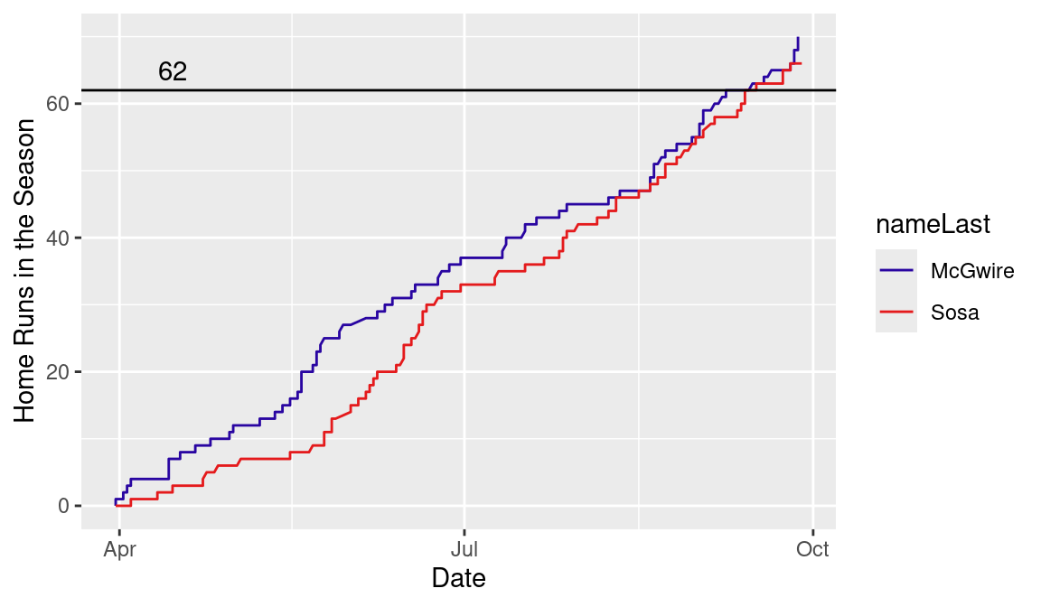
From the figure, we see that for much of the season, McGwire was the only man in the chase. Then Sosa caught fire and the two were very close in home runs starting from mid-August. “Big Mac” first broke the record, hitting his 62nd home run on September 8. Then, on September 25, the two were tied at 66 apiece. Finally, McGwire managed to hit four more in the final days of the season, while “Slammin’ Sammy” remained at 66.
To produce the graph in Figure 1.2 and relive the 1998 season, one needs data at a game-by-game level.
1.3.2 Retrosheet
Retrosheet is a volunteer organization, founded in 1989 by University of Delaware professor David Smith, that aims to collect play-by-play accounts of every game played in Major League Baseball history. Through the labor of love of many volunteers who have unearthed old newspaper accounts, scanned microfilms, and manually entered data into computers, the Retrosheet website4 contains game-by-game summaries going back to the dawn of Major League Baseball in the 19th century. The Retrosheet site also has play-by-play data of most of the games played since the 1913 season and continues to add games for previous seasons. These data are introduced in Section 1.4.
1.3.3 Game logs
Retrosheet provides individual game data going back to 1871. A game log has details regarding when the game was played, how many spectators attended, the teams and the ballpark, and the score (both the final score and the inning by inning runs scored). In addition, the game log file includes teams’ offensive and defensive statistics, starting players, managers, and umpire crews. There are missing observations for some game log variables for earlier baseball seasons.
Retrosheet provides a comprehensive Guide to Retrosheet Game Logs5 document that gives details of all 161 fields compiled for each game. Readers are encouraged to peruse the guide to fully understand the contents of the files. Details on the relevant data fields will be described when they are used in later chapters.
1.3.4 Obtaining the game logs from Retrosheet
Game log files can be found at https://www.retrosheet.org/gamelogs/index.html. A zip file is provided for each season, starting from 1871, and can be downloaded in a folder of choice by clicking on the relevant year. When one extracts the zip file, one obtains a plain text file (.txt extension) where fields are separated by commas. Section 11.4 provides an R function for downloading and parsing game log files.
1.3.5 Game log example
On September 9, 1995, Cal Ripken, Jr. of the Baltimore Orioles surpassed the seemingly unbeatable consecutive games record of 2130 belonging to the late Lou Gehrig. One can learn more about this historic game by exploring the game log files for the 1995 season. Table 1.6 contains a subset of the copious information available for this particular game between Baltimore and California. These data are taken from a single line in the gl1995.txt file available at https://www.retrosheet.org/gamelogs/index.html. This table displays team statistics6 as well as the players’ identities and fielding positions for the home team; similar statistics and player information are available for the visiting team.
| Variable | Value |
|---|---|
| date | 19950906 |
| dayofweek | Wed |
| visitorteam | CAL |
| hometeam | BAL |
| visitorrunsscored | 2 |
| homerunsscore | 4 |
| daynight | N |
| parkid | BAL12 |
| attendance | 46272 |
| duration | 215 |
| visitorlinescore | 100000010 |
| homelinescore | 10020010x |
| homeab | 34 |
| homeh | 9 |
| homehr | 4 |
| homerbi | 4 |
| homebb | 1 |
| homek | 8 |
| homegdp | 0 |
| homelob | 7 |
| homepo | 27 |
| homea | 8 |
| homee | 0 |
| umpirehname | Larry Barnett |
| umpire1bname | Greg Kosc |
| umpire2bname | Dan Morrison |
| umpire3bname | Al Clark |
| visitormanagername | Marcel Lacheman |
| homemanagername | Phil Regan |
| homestartingpitchername | Mike Mussina |
| homebatting1name | Brady Anderson |
| homebatting1position | 8 |
| homebatting2name | Manny Alexander |
| homebatting2position | 4 |
| homebatting3name | Rafael Palmeiro |
| homebatting3position | 3 |
| homebatting4name | Bobby Bonilla |
| homebatting4position | 9 |
| homebatting5name | Cal Ripken |
| homebatting5position | 6 |
| homebatting6name | Harold Baines |
| homebatting6position | 10 |
| homebatting7name | Chris Hoiles |
| homebatting7position | 2 |
| homebatting8name | Jeff Huson |
| homebatting8position | 5 |
| homebatting9name | Mark Smith |
| homebatting9position | 7 |
What does one learn from this game log information displayed in Table 1.6? This game took place on a Wednesday night in front of 46,272 people in Baltimore (the hometeam = BAL indicates the Orioles were the home team). The game lasted over three and a half hours (duration = 215 minutes), thanks in part to the standing ovation Ripken got at the end of the fifth inning, when the game became official. (The standing ovation information is not available in this file.) Baltimore defeated California 4-2; since we observe homehr = 4, we observe that all of Baltimore’s runs this game were due to four home runs with the bases empty. The Orioles infield in this game included Rafael Palmeiro at first base, Manny Alexander at second base, Ripken at shortstop, and Jeff Huson at third base.
1.3.6 Baseball questions
Here are some typical questions one can answer with the Retrosheet game logs files.
[Q] In which months are home runs more likely to occur? What about ballparks?
[A] Since 1980, July has been the month with the most home runs per game (1.97), while September has had the lowest frequency (1.84). In the same time frame, 2.71 home runs per game have been hit in Coors Field (home of the Colorado Rockies, and 1.14 in the Astrodome (the former home of the Houston Astros.
[Q] Do runs happen more frequently when some umpires are behind the plate? What is the difference between the most pitcher-friendly and the most hitter-friendly umpires?
[A] Among umpires with more than 400 games called since 1980, teams scored the highest number of runs (10.0 per game combined) when Chuck Meriwether was behind the plate and the lowest (7.8) when Doug Harvey was in charge.
[Q] How many extra people attend ballgames during the weekend? What’s the average attendance by day of the week?
[A] Close to 33,000 people attend games played on Saturdays (data from 1980 to 2011) and 31,000 on Sundays. The average goes down to 29,000 on Fridays, 25,000 on Thursdays and Mondays, and 24,000 on Tuesdays and Wednesdays.
1.4 Retrosheet Play-by-Play Data
1.4.1 Event files
Retrosheet has collected data to an even finer detail for most games played since 1913. For those seasons, play-by-play accounts are available at https://www.retrosheet.org/game.htm. These “event files” (as these play-by-play files are named) contain information on every single event happening on the field during a game. For each play, information is reported on the situation (inning, team batting, number of outs, presence of runners on base), the players on the field, the sequence of pitches thrown, and details on the play itself. For example, the file indicates whether a hit occurred, and if a ball in play is a ground ball, the file gives the defender that fielded the ball.
Event files come in a format expressly devised for them. Retrosheet gives detailed instruction on how to use the files7 and a step-by-step guide8, plus the software to parse the files.9 However, the process of rendering the files in a format suitable for use in R (or other statistical programs) is not straightforward without use of additional tools. Thus, in Appendix A, we present R code that implements the full process of downloading, extracting, and parsing these data. We also provide sample code to create the datasets used in this book.
1.4.2 Event example
Just as we use a historical game for the purpose of showing the contents of Retrosheet game logs, we use a famous fielding play to illustrate the Retrosheet event files. This play is represented as a single line in an event file shown in Table 1.7.
| Variable | Value |
|---|---|
| GAME_ID | OAK200110130 |
| YEAR_ID | 2001 |
| AWAY_TEAM_ID | NYA |
| INN_CT | 7 |
| BAT_HOME_ID | 1 |
| OUTS_CT | 2 |
| BALLS_CT | 2 |
| STRIKES_CT | 2 |
| PITCH_SEQ_TX | CSBBFX |
| AWAY_SCORE_CT | 1 |
| HOME_SCORE_CT | 0 |
| BAT_ID | longt002 |
| BAT_HAND_CD | L |
| PIT_ID | mussm001 |
| PIT_HAND_CD | R |
| POS2_FLD_ID | posaj001 |
| POS3_FLD_ID | martt002 |
| POS4_FLD_ID | soria001 |
| POS5_FLD_ID | bross001 |
| POS6_FLD_ID | jeted001 |
| POS7_FLD_ID | knobc001 |
| POS8_FLD_ID | willb002 |
| POS9_FLD_ID | spens001 |
| BASE1_RUN_ID | giamj002 |
| BASE2_RUN_ID | NA |
| BASE3_RUN_ID | NA |
| EVENT_TX | D9/9S.1XH(962) |
| BAT_FLD_CD | 7 |
| BAT_LINEUP_ID | 7 |
The play took place in a game played in Oakland on October 13, 2001, as can be inferred from the value of the GAME_ID variable. This game was Game 3 of the American League Division Series featuring the hometown Athletics against the New York Yankees (AWAY_TEAM_ID = NYA). The play occurred in the seventh inning with the home team batting (variables INN_CT and BAT_ID_ID). There were two outs (variable OUTS_CT) and the A’s were leading 1-0 (variables AWAY_SCORE_CT and HOME_SCORE_CT). Right-handed Mike Mussina (variables PIT_ID and PIT_HAND_CD) was on the mound for the Yankees, facing left-handed batter Terrence Long (variables BAT_ID and BAT_HAND_CD) with Jeremy Giambi standing on first base (variable BASE1_RUN_ID). The BAT_FLD_CD = 7 and BAT_LINEUP_ID = 7 fields inform us that Giambi’s defensive position was left field (position 7 corresponding to left field) and he was batting 7th in the lineup. The variables POS2_FLD_ID through POS9_FLD_ID report the full defensive lineup for the Yankees.
The seemingly inscrutable characters appearing in the PITCH_SEQ_TX and EVENT_TX variables depict what happened during that particular at bat. From looking at the pitch sequence variable PITCH_SEQ_TX, one sees that Mussina quickly went ahead in the count as Long let a strike go by and swung and missed at another pitch (CS). Then Mussina followed with consecutive balls (BB) and Long battled with a foul ball (F) before putting the ball in play (X). The variable EVENT_TX gives the results of the play. Long’s hit resulted in a double, collected by the Yankees right fielder (D9 in EVENT_TX) in short right (9S). The runner on first was thrown out on his way to home (1XH) by a throw from right fielder Shane Spencer, relayed by shortstop Derek Jeter to catcher Jorge Posada (962).
Once the event files are properly processed, many more fields are available than the ones presented in Table 1.7. However these additional fields are, for the most part, derived from what is in the table. For example, one additional field indicates whether the at-bat resulted in a base hit, one field will identify the fielder who collected the ball, and four fields will indicate where each runner (and the batter) stood at the end of the play—all of this can be inferred by the EVENT_TX field.
This play-by-play information is available for most games going back to 1913; thus it is possible to recreate what happened on the field in the past century. For this particular play, the Retrosheet event files cannot tell us all of the interesting details. Derek Jeter came out of nowhere to cut off Spencer’s throw and flipped it backhand to Posada in time to nail Giambi at home, on what has become known as “The Flip Play”.10
1.4.3 Baseball questions
Below are some questions that can be explored with the Retrosheet event files. These specific questions are about how batters perform in particular situations in the pitch count and with runners on base.
[Q] During the McGwire/Sosa home run race, which player was more successful at hitting homers with men on base?
[A] Mark McGwire hit 37 home runs in 313 plate appearances with runners on base, while Sammy Sosa hit 29 in 367. Once walks (both intentional and unintentional) and hit by pitches are removed, the number of opportunities become 223 for McGwire and 317 for Sosa.
[Q] How many intentional walks in unusual situations (e.g., empty bases or bases loaded) was Barry Bonds issued in his 73 HR campaign?
[A] During his record 2001 season, Barry Bonds was passed intentionally only 35 times. Of those free passes, one came with a runner on first and two with runners on first and second. When he was awarded 120 intentional walks in 2004, 19 came with nobody on, 11 with a runner on first, and 3 with runners on first and third. He was once walked intentionally with the bases loaded in 1998.
[Q] What is the Major league batting average when the ball/strike count is 0-2? What about on 2-0?
[A] In 2011, hitters compiled a .253 batting average on plate appearances where they fell behind 0-2. Conversely they hit .479 after going ahead 2-0.
1.5 Pitch-by-Pitch Data
1.5.1 MLBAM Gameday and PITCHf/x
Erstwhile Miami Marlins rightfielder Giancarlo Stanton emerged in 2017 as an elite slugger by blasting a league leading 59 balls out of the park. Figure 1.3 shows the location and the type of the 59 pitches Stanton sent into the stands.

Since 2005, baseball fans have had the opportunity to follow, pitch-by-pitch, the games played by their favorite team on the Web thanks to the Major League Baseball Advanced Media (MLBAM) Gameday application featured on the MLB.com website. For a couple of years, fans would only know the outcome of each pitch (whether it was a ball, a called strike, a swinging strike, and so on). Starting from an October 2006 game played at the Metrodome in Minneapolis, a wealth of detail began to appear for each pitch tracked on Gameday. Data on the release point, the pitch speed, and its full trajectory, were available for about one-third of the games played in 2007. Starting from the 2008 season, nearly every MLB pitch flight has been recorded by the PITCHf/x system. However, since the second edition of this book, PITCHf/x has been superseded by Statcast, a data source which is detailed in Section 1.6.1. What we provide here serves two purposes: first, it provides historical continuity; and second, most of the information recorded by PITCHf/x appears in a similar format in the Statcast data, so the content is still relevant. Unfortunately, we are not aware of a currently usable method for obtaining pitch-by-pitch data for the pre-Statcast period. Please see Appendix B for a fuller discussion of the rise and fall of PITCHf/x.
1.5.2 PITCHf/x Example
On April 21, 2012, Phil Humber became the 21st pitcher in Major League Baseball history to throw a perfect game by retiring all the 27 batters he faced. PITCHf/x captured his final pitch (like it did for nearly every other pitch thrown in MLB ballparks from 2008 to 2015), providing the data shown in Table 1.8. The outcome of the pitch (variable des) is recorded by a stringer (a human being), while most of the remaining information is either captured by the Sportvision camera system or calculated from the captured data.
| Variable | Value |
|---|---|
| des | Swinging Strike (Blocked) |
| sv_id | 120421_152537 |
| start_speed | 85.3 |
| end_speed | 79.1 |
| sz_top | 3.73 |
| sz_bot | 1.74 |
| pfx_x | 0.31 |
| pfx_z | 1.81 |
| px | 2.211 |
| pz | 1.17 |
| x0 | -1.58 |
| y0 | 50.0 |
| z0 | 5.746 |
| vx0 | 9.228 |
| vy0 | -124.71 |
| vz0 | -5.311 |
| ax | 0.483 |
| ay | 25.576 |
| az | -29.254 |
| break_y | 23.8 |
| break_angle | -4.1 |
| break_length | 7.8 |
| pitch_type | SL |
| spin_dir | 170.609 |
| spin_rate | 344.307 |
Each pitch is assigned an identifier (sv_id), that is actually a time stamp: Humber’s final pitch was recorded on April 21, 2012, at 15:25:37. The key information Sportvision obtains through its camera system is recorded in lines 11 through 19 of the table. Those nine parameters give the position (variables x0, y0, z0), velocity (variables vx0, vy0, vz0), and acceleration (variables ax, ay, az) components of the pitch at release point. With these nine parameters the full trajectory of the pitch from release to home plate can be estimated. (In fact, Sportvision actually estimates the parameters somewhere in the middle of the ball’s flight, then derives the parameters at release point.)
While the nine parameters just mentioned are sufficient for learning about the trajectory of the pitch, they are difficult to understand by casual fans who follow the game on MLBAM Gameday. Other more descriptive quantities are calculated starting from those nine parameters. The one measure familiar to baseball fans is the pitch speed at release, which for Humber’s final pitch is calculated at 85.3 mph (variable start_speed). PITCHf/x also provides the speed of the ball as it crosses the plate, 79.1 mph in this case (variable end_speed). Another two important values are the variables px and pz; they represent the horizontal and vertical location of the pitches, respectively, and can be combined with the batter’s strike zone upper and lower limits (sz_top and sz_bot) to infer whether the pitch crossed the strike zone.
Let’s focus on the location of this particular pitch. The horizontal reference point is the middle of the plate, with positive values indicating pitches passing on the right side of it from the umpire’s viewpoint. In this case the ball crossed the plate 2.21 feet on the right of its midpoint. Since the plate is 17 inches wide, it was way out of the strike zone. The pitch was also too low to be a strike, as the vertical point at which it crossed the plate is listed at 1.17 feet, while the hitter’s lower limit of the strike zone is 1.74.11 Luckily for Humber (since otherwise a walk would have ruined the perfect game), the home plate umpire controversially declared that Brendan Ryan had swung the bat for strike three.
Other interesting quantities about a pitch are available with PITCHf/x, including the horizontal and vertical movement (variables pfx_x and pfx_z) of the pitch trajectory, the spin direction, and its spin rate (variables spin_dir and spin_rate). MLBAM has devised a complex algorithm that processes the information captured by Sportvision and marks the pitch with a label familiar to baseball fans. In this case the algorithm recognizes the pitch as a slider (variable pitch_type).
1.5.3 Baseball questions
Below are questions you can answer with PITCHf/x data. The data can be used to address specific questions about pitch type, speed of the pitch, and play outcomes on specific pitches.
[Q] Who are the hitters who see the lowest and the highest percentage of fastballs?
[A] From 2008 to 2011, pitchers have thrown fastballs 35% of the time when Ryan Howard was at the plate, 56% of the time when facing David Eckstein.
[Q] Who is the fastest pitcher in baseball currently?
[A] Nine of the fastest ten pitches recorded by PITCHf/x from 2008 to 2011 have been thrown by Aroldis Chapman, the highest figure being a 105.1 mph pitch thrown on September 24, 2010 in San Diego. Neftali Feliz is the other pitcher making the top ten list with a 103.4 fastball delivered in Kansas City on September 1, 2010.
[Q] What are the chances of a successful steal when the pitcher throws a fastball compared to when a curve is delivered?
[A] From 2008 to 2010, baserunners were successful 73% of the times at stealing second base on a fastball. The success rate increases to 85% when the pitch is a curveball.
1.6 Player Movement and Off-the-Bat Data
1.6.1 Statcast
Statcast is a new technology that tracks movements of all baseball players and the baseball during a game. It was introduced to all MLB stadiums in 2015, and all teams have access to the large amount of data collected. Some of the Statcast data for pitchers and hitters is currently publicly available via the Baseball Savant website. Also, these data are used during a baseball broadcast for entertainment purposes. For example, a baseball announcer will provide the launch angle, exit velocity, and distance traveled for a home run. The broadcast will give the distance that an outfielder moves towards a batted ball and the speed of a baserunner from home to first base.
1.6.2 Baseball Savant data
To illustrate the new information available from Statcast, consider data on one of the hardest hit home runs during the 2018 season. In a game between the New York Yankees at the Toronto Blue Jays on June 6, 2018, Giancarlo Stanton of the Yankees hit a home run in the top of the 13th inning. The baseballr package provides a function to download data on each pitch from the Baseball Savant website, and Table 1.9 displays a number of variables for this specific home run.
| Variable | Value |
|---|---|
| pitch_type | CH |
| game_date | 2018-06-06 |
| release_speed | 85.4 |
| batter | 519317 |
| pitcher | 607352 |
| events | home_run |
| des | Giancarlo Stanton homers (14) on a line drive to left field. |
| home_team | TOR |
| away_team | NYY |
| balls | 1 |
| strikes | 0 |
| game_year | 2018 |
| plate_x | -0.2197 |
| plate_z | 2.4995 |
| outs_when_up | 2 |
| inning | 13 |
| inning_topbot | Top |
| hc_x | 20.36 |
| hc_y | 56.47 |
| hit_distance_sc | 416 |
| launch_speed | 119.3 |
| launch_angle | 15.044 |
| pitch_name | Changeup |
| home_score | 0 |
| away_score | 2 |
| if_fielding_alignment | Standard |
| of_fielding_alignment | Standard |
| barrel | 1 |
The batter id and pitcher id are respectively 519317 and 607352 which correspond to Giancarlo Stanton and Joe Biagini. The game situation variables are inning, inning_topbot, outs_when_up, home_score, away_score, balls, and strikes. We learn that this home run was hit in the top of the 13th inning when the Yankees were leading 2-0, there were two outs, and the count was 1-0.
The variables if_fielding_alignment and of_fielding_alignment relate to the positioning of the Toronto fielders for this particular pitch. Both variables are “Standard”, which indicate that there was no special shifting of the infielders or outfielders for Stanton for this particular at-bat.
Other variables give characteristics of the pitch. The pitch_type and pitch_name variables indicate that the pitch was a change-up thrown at a release_speed of 85.4 mph. The plate_x and plate_y variables give the location of the pitch—these values indicate that the pitch was located in the middle of the zone.
This dataset also includes characteristics of the batted ball. The launch_speed and launch_angle variables tell us that the ball came off of the bat at a speed of 119.3 mph at a launch angle of 15.044 degrees. It is notable that this particular batted ball was a line drive—it must have been hit hard for a home run. The hit_distance_sc variable indicates that the ball was hit a distance of 416 feet. The hc_x and hc_y variables tell us about the direction (more specifically, the spray angle of this home run).
More details about the Statcast data and how to use it appear in Appendix C.
1.6.3 Baseball questions
The following questions can be addressed with Statcast data.
[Q] What is a typical launch speed and launch angle of a home run?
[A] Using 2017 season data, the median launch speed of a home run was 103 mph and the median launch angle was 27.8 degrees.
[Q] How frequently do MLB teams employ infield shifts?
[A] Using data from the first part of the 2018 season, teams employed an infield shift or some strategic infield defense for 26 percent of the batters.
[Q] Is an infield shift effective in defensing ground balls?
[A] Using data from the 2018 season, the batting average on ground balls with a standard infield defense was 0.281, and with an infield shift the batting average on ground balls dropped to 0.231.
1.7 Data Used in this Book
We use data from all four of the sources above in various places in this book. Generally, data that comes from the Lahman database will be accessed directly from the R package Lahman. Small data sets are available through the abdwr3edata package, the full source of which is located on GitHub. The Retrosheet and Statcast data is large enough that it is generally not included in the GitHub repositories. In order to reproduce the results in this book using those datasets, you will need to download those data on your own. Instructions for doing so appear in Section A.1.3 (for Retrosheet) and Section 12.2 (for Statcast).
1.8 Summary
When choosing among the four main sources of baseball data (Lahman, Retrosheet, PITCHf/x, and Statcast, one always has to consider the trade-off between the level of detail and the seasons covered by the source. With Lahman’s database, for example, one can explore the evolution of the game since its beginnings back into the 19th century. However, only the basic season count statistics are available from this source. For example, simple information such as Babe Ruth’s batting splits by pitcher’s handedness cannot be retrieved from Lahman’s files.
Retrosheet is steadily adding past seasons to its play-by-play database, allowing researchers to perform studies to validate or reject common beliefs about players of the past decades. During the years, for example, analysis of play-by-play data has confirmed the huge defensive value of players like Brooks Robinson and Mark Belanger, and has substantiated the greatness of Roberto Clemente’s throwing arm.
PITCHf/x was available from 2008–2015 and, unlike with Retrosheet, there is no way to compile data for games of the past. This means we will never be able to compare the velocity of Aroldis Chapman’s fastball to that of Nolan Ryan or Bob Feller. However, studies performed since its inception have provided an enhanced understanding of the game, enabling researchers to explore issues like pitch sequencing, batter discipline, pitcher fatigue, catcher framing (see Chapter 7) and the catcher’s ability to block bad pitches.
Statcast represents the newest wave of baseball data. Since it includes detailed information on the positioning and movement of players, it has been useful in evaluating the effectiveness of a fielder in reaching a batted ball and understanding the performance of runners on the bases. Also, Statcast has helped us understand the relationship between the batted ball variables (launch angle, exit velocity, and spray angle and base hits and outs.
1.9 Further Reading
Schwarz (2004) provides a detailed history of baseball statistics. Adler (2006) explains how to obtain baseball data from several sources, including Lahman’s database, Retrosheet, and MLBAM Gameday and how to analyze them using diverse tools, from Microsoft Excel to R, MySQL, and PERL. Fast (2010) introduces the PITCHf/x system to the uninitiated. The PITCHf/x, HITf/x, FIELDf/x section of The Physics of Baseball website (http://baseball.physics.illinois.edu/) features material on the subject of pitch tracking data.
1.10 Exercises
1. Which Datafile?
This chapter has given an overview of the Lahman database, the Retrosheet game logs, the Retrosheet play-by-play files, the PITCHf/x database, and the Statcast database. Describe the relevant data among these four databases that can be used to answer the following baseball questions.
- How has the rate of walks (per team for nine innings) changed over the history of baseball?
- What fraction of baseball games in 1968 were shutouts? Compare this fraction with the fraction of shutouts in the 2012 baseball season.
- What percentage of first pitches are strikes? If the count is 2-0, what fraction of the pitches are strikes?
- Which players are most likely to hit groundballs? Of these players, compare the speeds at which these groundballs are hit.
- Is it easier to steal second base or third base? (Compare the fraction of successful steals of second base with the fraction of successful steals of third base.)
2. Lahman Pitching Data
From the pitching data file from the Lahman database, the following information is collected about Bob Gibson’s famous 1968 season.
NA    playerID yearID stint teamID lgID  W L  G GS CG SHO SV
NA 1 gibsobo01   1968     1    SLN   NL 22 9 34 34 28  13  0
NA   IPouts   H ER HR BB  SO BAOpp  ERA IBB WP HBP BK  BFP GF  R
NA 1    914 198 38 11 62 268  0.18 1.12   6  4   7  0 1161  0 49
NA   SH SF GIDP
NA 1 NA NA NA- Gibson started 34 games for the Cardinals in 1968. What fraction of these games were completed by Gibson?
- What was Gibson’s ratio of strikeouts to walks this season?
- One can compute Gibson’s innings pitched by dividing
IPoutsby three. How many innings did Gibson pitch this season? - A modern measure of pitching effectiveness is WHIP, the average number of hits and walks allowed per inning. What was Gibson’s WHIP for the 1968 season?
3. Retrosheet Game Log
Jim Bunning pitched a perfect game on Father’s Day on June 21, 1964. Some details about this particular game can be found from the Retrosheet game logs.
NA       Date DoubleHeader DayOfWeek VisitingTeam
NA 1 19640621            1       Sun          PHI
NA   VisitingTeamLeague VisitingTeamGameNumber HomeTeam
NA 1                 NL                     60      NYN
NA   HomeTeamLeague HomeTeamGameNumber VisitorRunsScored
NA 1             NL                 67                 6
NA   HomeRunsScore LengthInOuts DayNight CompletionInfo
NA 1             0           54        D             NA
NA   ForfeitInfo ProtestInfo ParkID Attendance Duration
NA 1          NA              NYC17          0      139
NA   VisitorLineScore HomeLineScore VisitorAB VisitorH VisitorD
NA 1        110004000     000000000        32        8        2
NA   VisitorT VisitorHR VisitorRBI VisitorSH VisitorSF VisitorHBP
NA 1        0         1          6         2         0          0
NA   VisitorBB VisitorIBB VisitorK VisitorSB VisitorCS VisitorGDP
NA 1         4          0        6         0         1          0
NA   VisitorCI VisitorLOB
NA 1 0 5- What was the time in hours and minutes of this particular game?
- Why is the attendance value in this record equal to zero?
- How many extra base hits did the Phillies have in this game? (We know that the Mets had no extra base hits this game.)
- What was the Phillies’ on-base percentage in this game?
4. Retrosheet Play-by-Play Record
One of the famous plays in Philadelphia Phillies history is second baseman Mickey Morandini’s unassisted triple play against the Pirates on September 20, 1992. The following records from the Retrosheet play-by-play database describe this half-inning. The variables indicate the half-inning (variables INN_CT and HOME_ID), the current score (variables AWAY_SCORE_CT and HOME_SCORE_CT), the identities of the pitcher and batter (variables BAT_ID and PIT_ID), the pitch sequence (variable PITCH_SEQ), the play event description (variable EVENT_TEX), and the runners on base (variables BASE1_RUN and BASE2_ID).
NA   bat_home_id away_score_ct home_score_ct   bat_id   pit_id
NA 1           1             1             1 vansa001 schic002
NA 2           1             1             1 bondb001 schic002
NA 3           1             1             1 kingj001 schic002
NA   pitch_seq_tx event_cd             event_tx base1_run_id
NA 1        CBBBX       20               S9/L9M
NA 2         C1BX       20            S/G56.1-2     vansa001
NA 3       BLLBBX        2 4(B)4(2)4(1)/LTP/L4M     bondb001
NA   base2_run_id
NA 1
NA 2
NA 3     vansa001
Based on the records, write a short paragraph that describes the play-by-play events of this particular inning.
5. PITCHf/x Record of Several Pitches
R.A. Dickey was one of the few current pitchers in recent years who threw a knuckleball. The following gives some PITCHf/x variables for the first knuckleball and the first fastball that Dickey threw for a game against the Kansas City Royals on April 13, 2013.
start_speed end_speed pfx_x pfx_z     px    pz sz_bot sz_top
         73      66.3 -0.64 -7.58 -0.047 2.475    1.5   3.35

start_speed end_speed pfx_x pfx_z    px    pz sz_bot sz_top
       81.2      75.4 -4.99 -7.67 -1.99 2.963    1.5   3.43
Describe the differences between the knuckleball and the fastball in terms of pitch speed, movement (horizontal and vertical directions), and location in the strike zone. Based on this data, why is a knuckleball so difficult for a batter to make contact?
Examples of people who never played Major League Baseball but have been inducted into the Hall of Fame (therefore having an entry in the
Peopletable) are baseball pioneer Henry Chadwick and career Negro Leaguer Josh Gibson.↩︎See Chapter 11 for an introduction to park factors.↩︎
Some other team statistics omitted in Table 1.6—such as Stolen Bases and Caught Stealing—are reported in game log files.↩︎
How to use Our Event Files: https://www.retrosheet.org/datause.txt↩︎
Step-by-Step Example: https://www.retrosheet.org/stepex.txt↩︎
Software Tools: https://www.retrosheet.org/tools.htm↩︎
In 2002, Baseball Weekly recognized “The Flip Play” as one of the ten most amazing fielding plays of all time.↩︎
The batter’s strike zone boundaries are recorded by the human stringer at the beginning of the at-bat, and thus are less precise than the pitch location coordinates recorded by the advanced system.↩︎