9 Simulation

9.1 Introduction
A baseball season consists of a collection of games between teams, where each game consists of nine innings, and a half-inning consists of a sequence of plate appearances. Because of this clean structure, the sport can be represented by relatively simple probability models. Simulations from these models are helpful in understanding different characteristics of the game.
One attractive aspect of the R system is its ability to simulate from a wide variety of probability distributions. In this chapter, we illustrate the use of R functions to simulate a game consisting of a large number of plate appearances. Also, we use R to simulate the game-to-game competition between teams during an entire season.
Section 9.2 focuses on simulating the events in a baseball half-inning using a special probability model called a Markov chain. The runners on base and the number of outs define a state and this probability model describes movements between states until one reaches three outs. The movement or transition probabilities are found using actual data from the 2016 season. By simulating many half-innings using this model, one gets a basic understanding of the pattern of run scoring.
Section 9.3 describes a simulation of an entire baseball season using the Bradley-Terry probability model. Teams are assigned talents from a bell-shaped (normal) distribution and a season of baseball games is played using win probabilities based on the talents. By simulating many seasons, one learns about the relationship between a team’s talent and its performance in a 162-game season. We describe simulating the post-season series and assess the probability that the “best” team, that is, the team with the best ability actually wins the World Series.
9.2 Simulating a Half Inning
9.2.1 Markov chains
A Markov chain is a special type of probability model useful for describing movement between locations, called states. In the baseball context, a state is viewed as a description of the runners on base and the number of outs in an inning. Each of the three bases can be occupied by a runner or not, and so there are 2 \(\times\) 2 \(\times\) 2 = 8 possible runner situations. Since there are three possible numbers of outs (0, 1, or 2), there are 8 \(\times\) 3 = 24 possible runner and outs states. If we include the 3 outs state, there are a total of 25 possible states during a half-inning of baseball (see Section 5.1).
In a Markov chain, a matrix of transition probabilities is used to describe how one moves between the different states. For example, suppose that there are currently runners on first and second with one out. Based on the outcome of the plate appearance, the state can change. For example, the batter may hit a single; the runner on second scores and the runner on first moves to third. In this case, the new state is runners on first and third with one out. Or maybe the batter will strike out, and the new state is runners on first and second with two outs. By looking at a specific row in the transition probability matrix, one learns about the probability of moving to first and third with one out, or moving to first and second with two outs, or any other possible state.
In a Markov chain, there are two types of states: transition states and absorbing states. Once one moves into an absorbing state, one remains there and can’t return to other transition states. In a half-inning of baseball, since the inning is over when there are 3 outs, this 3-outs state acts as an absorbing state.
There are some special assumptions in a Markov chain model. We assume that the probability of moving to a new state only depends on the current state. So any baseball events that happened before the current runners and outs situation are not relevant in finding the probabilities1. In other words, this model assumes there is not a momentum effect in batting through an inning. Also we are assuming that the probabilities of these movements are the same for all teams, against all pitchers, and for all innings during a game. Clearly, this assumption that all teams are average is not realistic, but we will address this issue in one of the other sections of this chapter.
There are several attractive aspects of using a Markov chain to model a half-inning of baseball. First, the construction of the transition probability matrix is easily done with 2016 season data using computations from Chapter 5. One can use the model to play many half-innings of baseball, and the run scoring patterns that are found resemble the actual run scoring of actual MLB baseball. Last, there are special properties of Markov chains that simplify some interesting calculations, such as the number of players who come to bat during an inning.
9.2.2 Review of work in run expectancy
To construct the transition matrix for the Markov chain, one needs to know the frequencies of transitions from the different runners/outs states to other possible runners/outs states. One can obtain these frequencies using the Retrosheet play-by-play data from a particular season. Here we review the work from Chapter 5.
We begin by reading in play-by-play data for the 2016 season, creating the data frame retro2016.
First, we use the retrosheet_add_states() function that we wrote in Chapter 5 and stored in the abdwr3edata package. This function adds a number of useful new variables to retro2016. Recall that in particular, we now have a new variable state (which gives the runner locations and the number of outs at the beginning of each play), and a another new variable new_state (which contains the same information at the conclusion of the play).
library(abdwr3edata)
retro2016 <- retro2016 |>
  retrosheet_add_states()
Next, we create the variable half_inning_id as a unique identifier for each half-inning in each baseball game. The new variable runs gives the number of runs scored in each play. The new data frame half_innings contains data aggregated over each half-inning of baseball played in 2016.
half_innings <- retro2016 |>
  mutate(
    runs = away_score_ct + home_score_ct,
    half_inning_id = paste(game_id, inn_ct, bat_home_id)
  ) |>
  group_by(half_inning_id) |>
  summarize(
    outs_inning = sum(event_outs_ct),
    runs_inning = sum(runs_scored),
    runs_start = first(runs),
    max_runs = runs_inning + runs_start
  )
By using the filter() function from the dplyr package, we focus on plays where there is a change in the state or in the number of runs scored. By another application of filter(), we restrict attention to complete innings where there are three outs and where there is a batting event; the new dataset is called retro2016_complete. Here non-batting plays such as steals, caught stealing, wild pitches, and passed balls are ignored. There is obviously some consequence of removing these non-batting plays from the viewpoint of run production, and this issue is discussed later in this chapter.
In our definition of the new_state variable, we recorded the runner locations when there were three outs. The runner locations don’t matter, so we recode new_state to always have the value 3 when the number of outs is equal to 3. The str_replace() function replaces the regular expression [0-1]{3} 3—which matches any three character binary string followed by a space and a 3—with 3.
retro2016_complete <- retro2016_complete |>
  mutate(new_state = str_replace(new_state, "[0-1]{3} 3", "3"))
9.2.3 Computing the transition probabilities
Now that the state and new_state variables are defined, one can compute the frequencies of all possible transitions between states using the table() function. The matrix of counts is T_matrix. There are 24 possible values of the beginning state state, and 25 values of the final state new_state including the 3-outs state.
This matrix can be converted to a probability matrix by use of the prop.table() function. The resulting matrix is denoted by P_matrix.
P_matrix <- prop.table(T_matrix, 1)
dim(P_matrix)
NA [1] 24 25Finally, we add a row to this transition probability matrix corresponding to transitions from the 3-out state. When the inning reaches 3 outs, then it stays at 3 outs, so the probability of staying in this state is 1.
The matrix P_matrix now has two important properties that allow it to model transitions between states in a Markov chain: 1) it is square, and; 2) the entries in each of its rows sum to 1.
dim(P_matrix)NA [1] 25 25P_matrix |>
apply(MARGIN = 1, FUN = sum)NA 000 0 000 1 000 2 001 0 001 1 001 2 010 0 010 1 010 2 011 0
NA 1 1 1 1 1 1 1 1 1 1
NA 011 1 011 2 100 0 100 1 100 2 101 0 101 1 101 2 110 0 110 1
NA 1 1 1 1 1 1 1 1 1 1
NA 110 2 111 0 111 1 111 2 3
NA 1 1 1 1 1To better understand this transition matrix, we display the transition probabilities starting at the “000 0” state, no runners and no outs below. (Only the positive probabilities are shown and the as_tibble() and pivot_longer() functions are used to display the probabilities vertically.) The most likely transitions are to the “no runners, one out” state with probability 0.676 and to the “runner on first, no outs” state with probability 0.235. The probability of moving from the “000 0” state to the “000 0” state is 0.033; in other words, the chance of a home run with no runners on with no outs is 0.033.
P_matrix |>
  as_tibble(rownames = "state") |>
  filter(state == "000 0") |>
  pivot_longer(
    cols = -state,
    names_to = "new_state",
    values_to = "Prob"
  ) |>
  filter(Prob > 0)
NA # A tibble: 5 × 3
NA state new_state Prob
NA <chr> <chr> <dbl>
NA 1 000 0 000 0 0.0334
NA 2 000 0 000 1 0.676
NA 3 000 0 001 0 0.00563
NA 4 000 0 010 0 0.0503
NA 5 000 0 100 0 0.235Let’s contrast this with the possible transitions starting from the “010 2” state, runner on second with two outs. The most likely transitions are “3 outs” (probability 0.650), “runners on first and second with two outs” (probability 0.156), and “runner on first with 2 outs” (probability 0.074).
P_matrix |>
  as_tibble(rownames = "state") |>
  filter(state == "010 2") |>
  pivot_longer(
    cols = -state,
    names_to = "new_state",
    values_to = "Prob"
  ) |>
  filter(Prob > 0)
NA # A tibble: 8 × 3
NA state new_state Prob
NA <chr> <chr> <dbl>
NA 1 010 2 000 2 0.0233
NA 2 010 2 001 2 0.00587
NA 3 010 2 010 2 0.0576
NA 4 010 2 011 2 0.000451
NA 5 010 2 100 2 0.0745
NA 6 010 2 101 2 0.0325
NA 7 010 2 110 2 0.156
NA 8 010 2 3 0.6509.2.4 Simulating the Markov chain
One can simulate this Markov chain model a large number of times to obtain the distribution of runs scored in a half-inning of 2016 baseball. The first step is to construct a matrix giving the runs scored in all possible transitions between states. Let \(N_{runners}\) denote the number of runners in a state and \(O\) denote the number of outs. Because every player who has already batted in the inning is either on base, out, or has scored, for a batting play, the number of runs scored is equal to \[ runs = (N_{runners}^{(b)} + O^{(b)} + 1) - (N_{runners}^{(a)} + O^{(a)}). \]
In other words, the runs scored is the sum of runners and outs before (b) the play minus the sum of runners and outs after (a) the play plus one. For example, suppose there are runners on first and second with one out, and after the play, there is a runner on second with two outs. The number of runs scored is equal to \[ runs = (2 + 1 + 1) - (1 + 2) = 1. \]
We define a new function num_havent_scored() which takes a state as input and returns the sum of the number of runners and outs. We then apply this function across all the possible states (using the map_int() function) and the corresponding sums are stored in the vector runners_out.
The outer() function with the - (subtraction) operation performs the runs calculation for all possible pairs of states and the resulting matrix is stored in the matrix R_runs. If one inspects the matrix R_runs, one will notice some negative values and some strange large positive values. But this is not a concern since the corresponding transitions, for example a movement between a “000 0” state and a “000 2” state in one batting play, are not possible. To make the matrix square, we add an additional column of zeros to this run matrix using the cbind() function.
We are now ready to simulate a half-inning of baseball using a new function simulate_half_inning(). The inputs are the probability transition matrix P, the run matrix R, and the starting state s (an integer between 1 and 24). The output is the number of runs scored in the half-inning.
There are two key statements in this simulation. If the current state is s, the function sample() will simulate a new state using the s row in the transition matrix P; the new state is denoted s_new. The total number of runs scored in the inning is updated using the value in the s row and the s_new column of the runs matrix R.
Using the map_int() function, one can simulate a large number of half-innings of baseball. In the below code, we simulate 10,000 half-innings starting with no runners and no outs (state 1), collecting the runs scored in the vector simulated_runs. The set.seed() function sets the random number seed so the reader can reproduce the results of this particular simulation by running this code.
To find the possible runs scored in a half-inning, we use the table() function to tabulate the values in simulated_runs.
table(simulated_runs)NA simulated_runs
NA 0 1 2 3 4 5 6 7 8 9
NA 7364 1437 651 324 126 50 34 10 2 2In our 10,000 simulations, five or more runs scored in 50 + 34 + 10 + 2 + 2 = 98 half-innings, so the chance of scoring five or more runs would be 98 / 10,000 = 0.0098. This calculation can be checked using the sum() function.
sum(simulated_runs >= 5) / 10000NA [1] 0.0098We compute the mean number of runs scored by applying the mean() function to simulated_runs.
mean(simulated_runs)NA [1] 0.477Over the 10,000 half-innings, an average of 0.4773 runs were scored.
To understand the runs potential of different runners and outs situations, one can repeat this simulation procedure for other starting states. We write a function runs_j() to compute the mean number of runs scored starting with state j. Using the map_int() function, we apply the function runs_j() over all of the possible starting states 1 through 24. The output is a vector of mean runs scored stored in the mean_run_value column. These values are displayed below as a simulated expected run matrix (see Section 5.1).
runs_j <- function(j) {
  1:10000 |>
    map_int(~simulate_half_inning(T_matrix, R_runs, j)) |>
    mean()
}

erm_2016_mc <- tibble(
  state = row.names(T_matrix),
  mean_run_value = map_dbl(1:24, runs_j)
) |>
  mutate(
    bases = str_sub(state, 1, 3),
    outs_ct = as.numeric(str_sub(state, 5, 5))
  ) |>
  select(-state)

erm_2016_mc |>
  pivot_wider(names_from = outs_ct, values_from = mean_run_value)
NA # A tibble: 8 × 4
NA bases `0` `1` `2`
NA <chr> <dbl> <dbl> <dbl>
NA 1 000 0.481 0.255 0.103
NA 2 001 1.32 0.925 0.338
NA 3 010 1.14 0.640 0.295
NA 4 011 1.93 1.30 0.474
NA 5 100 0.855 0.500 0.211
NA 6 101 1.71 1.14 0.425
NA 7 110 1.39 0.875 0.406
NA 8 111 2.19 1.46 0.667Recall that our simulation model is based only on batting plays. To understand the effect of non-batting plays (stealing, caught stealing, wild pitches, etc.) on run scoring, we compare this run expectancy matrix with the one found in Chapter 5 using all batting and non-batting plays. Their difference is the contribution of non-batting plays to the average number of runs scored.
erm_2016 <- read_rds(here::here("data/erm2016.rds"))

erm_2016 |>
  inner_join(erm_2016_mc, join_by(bases, outs_ct)) |>
  mutate(
    run_value_diff = round(mean_run_value.x - mean_run_value.y, 2)
  ) |>
  select(bases, outs_ct, run_value_diff) |>
  pivot_wider(names_from = outs_ct, values_from = run_value_diff)
NA # A tibble: 8 × 4
NA # Groups: bases [8]
NA bases `0` `1` `2`
NA <chr> <dbl> <dbl> <dbl>
NA 1 000 0.02 0.01 0
NA 2 001 0.03 0.01 0.03
NA 3 010 0 0.03 0.02
NA 4 011 0 0.06 0.07
NA 5 100 0 0.01 0.01
NA 6 101 0.02 0.06 0.05
NA 7 110 0.06 0.05 0.01
NA 8 111 -0.08 0.07 0.03Note that most of the values of the difference are positive, indicating that these non-batting plays generally do create runs. We note that the largest values tend to occur in situations when there is a runner on third who can score on a wild pitch or passed ball.
9.2.5 Beyond run expectancy
By using properties of Markov chains, it is straightforward to use the transition matrix to learn more about the movement through the runners/outs states.
By multiplying the probability matrix P_matrix by itself three times, we can learn about the likelihood of the state of the inning after three plate appearances. In R, matrix multiplication is indicated by the %*% symbol. The result is stored in the matrix P_matrix_3.
The first row of P_matrix_3 gives the probabilities of being in each of the 25 states after three hitters starting at the “000 0” state. We round these values to three decimal places, sort from largest to smallest, and display the largest values.
P_sorted <- P_matrix_3 |>
  as_tibble(rownames = "state") |>
  filter(state == "000 0") |>
  pivot_longer(
    cols = -state, names_to = "new_state", values_to = "Prob"
  ) |>
  arrange(desc(Prob))
P_sorted |>
  slice_head(n = 6)
NA # A tibble: 6 × 3
NA state new_state Prob
NA <chr> <chr> <dbl>
NA 1 000 0 3 0.372
NA 2 000 0 100 2 0.241
NA 3 000 0 110 1 0.0815
NA 4 000 0 010 2 0.0739
NA 5 000 0 000 2 0.0529
NA 6 000 0 001 2 0.0286After three PAs, the most likely outcomes are three outs (probability 0.3722999), runner on first with 2 outs (probability 0.2408963), and runners on first and second with one out (probability 0.08148).
It is also easy to learn about the number of visits to all runner-outs states. Define the matrix Q to be the 24-by-24 submatrix found from the transition matrix by removing the last row and column (the three outs state). By subtracting the matrix Q from the identity matrix and taking the inverse of the result, we obtain the fundamental matrix N of an absorbing Markov chain. (The diag() function is used to construct the identity matrix and the function solve() takes the matrix inverse.)
To understand the fundamental matrix, we display the beginning entries of the first row of the matrix.
NA 000 0 000 1 000 2 001 0 001 1 001 2
NA  1.05  0.75  0.60  0.01  0.03  0.05
Starting at the beginning of the inning (the “000 0” state), the average number of times the inning will be in the “000 0” state is 1.05, the average number of times in the “000 1” state is 0.75, the average number of times in the “000 2” state is 0.6, and so on. By using the sum() function, we find the average number of states that are visited.
sum(N_0000)NA [1] 4.27In other words, the average number of plate appearances in a half-inning (before three outs) is 4.27.
We can compute the average number of batting plays until three outs for all starting states by multiplying the fundamental matrix N by a column vector of ones. The vector of average number of plays is stored in the variable avg_num_plays and eight values of this vector are displayed.
NA 000 0 000 1 000 2 001 0 001 1 001 2 010 0 010 1
NA  4.27  2.87  1.46  4.33  2.99  1.53  4.34  2.93
This tells us the length of the remainder of the inning, on average, starting with each possible state. For example, starting at the bases empty, one out state, we expect on average to have 2.87 more batters. In contrast, with a runner on third with two outs, we expect to have 1.53 more batters.
9.2.6 Transition probabilities for individual teams
The transition probability matrix describes movements between states for an average team. Certainly, these probabilities will vary for teams of different batting abilities, and the probabilities will also vary against teams of different pitching abilities. We focus on different batting teams and discuss how to obtain good estimates of the transition probabilities for all teams.
To get the relevant data, a new variable batting_team needs to be defined that gives the batting team in each half-inning. By use of the str_sub() function, we define the home team variable home_team_id, and an if_else() function is used to define the batting team.
By use of the group_by() and count() functions, we construct a data frame T_team giving the counts of each team in the transitions from the current to new states.
For example, the filtering for batting_team equal to ANA gives the transition counts for Anaheim in the 2016 season.
T_team |>
  filter(batting_team == "ANA") |>
  slice_head(n = 6)
NA # A tibble: 192 × 4
NA # Groups: batting_team, state, new_state [192]
NA batting_team state new_state n
NA <chr> <chr> <chr> <int>
NA 1 ANA 000 0 000 0 40
NA 2 ANA 000 0 000 1 1007
NA 3 ANA 000 0 001 0 9
NA 4 ANA 000 0 010 0 75
NA 5 ANA 000 0 100 0 359
NA 6 ANA 000 1 000 1 31
NA 7 ANA 000 1 000 2 720
NA 8 ANA 000 1 001 1 3
NA 9 ANA 000 1 010 1 54
NA 10 ANA 000 1 100 1 261
NA # ℹ 182 more rowsIf one is interested in comparing run productions for different batting teams, it is necessary to make some adjustments to the team transition probability matrices to get realistic predictions of performance. To illustrate the problem, we focus on transitions from the “100 2” state. We store the transition counts in the data frame T_team_S using the tally() function and display a few rows of this table below for six of the teams.
NA # A tibble: 6 × 4
NA   batting_team state new_state     n
NA   <chr>        <chr> <chr>     <int>
NA 1 MIN          100 2 010 2        15
NA 2 CIN          100 2 101 2        19
NA 3 NYN          100 2 101 2        14
NA 4 SEA          100 2 010 2         6
NA 5 DET          100 2 011 2         9
NA 6 DET          100 2 101 2        15
For some of the less common transitions, there is much variability in the counts across teams and this causes the corresponding team transition probabilities to be unreliable. If \(p^{TEAM}\) represents the team’s transition probabilities for a particular team, and \(p^{ALL}\) are the average transition probabilities, then a better estimate at the team’s probabilities has the form \[ p^{EST} = \frac{n}{n + K} p^{TEAM} + \frac{K}{n + K} p^{ALL}, \] where \(n\) is the number of transitions for the team and \(K\) is a smoothing count. The description of the methodology is beyond the scope of this book, but in this case a smoothing count of \(K = 1274\) leads to a good estimate at the team’s transition probabilities. (The choice of \(K\) depends on the starting state.)
This method is illustrated for Washington’s transition counts starting from the “100 2” state. In the data frame T_WAS, the transition counts are stored in the variable n, and the corresponding proportions are stored in p. Similarly, for all teams, n and p are the counts and proportions in the data frame T_all.
We compute the improved estimate at Washington’s transition proportions using the formula and store the results in p_EST. The three sets of proportions (Washington, overall, and improved) are displayed in a data frame.
T_WAS |>
  inner_join(T_all, by = "new_state") |>
  mutate(
    p_EST = (n.x / (1274 + n.x)) * p.x + (1274 / (1274 + n.x)) * p.y
  )  |>
  select(batting_team, new_state, p.x, p.y, p_EST)
NA # A tibble: 8 × 6
NA # Groups: batting_team, state [1]
NA state batting_team new_state p.x p.y p_EST
NA <chr> <chr> <chr> <dbl> <dbl> <dbl>
NA 1 100 2 WAS 000 2 0.0319 0.0291 0.0291
NA 2 100 2 WAS 001 2 0.00532 0.00577 0.00577
NA 3 100 2 WAS 010 2 0.0213 0.0220 0.0219
NA 4 100 2 WAS 011 2 0.0213 0.0220 0.0219
NA 5 100 2 WAS 100 2 0.00266 0.000775 0.000776
NA 6 100 2 WAS 101 2 0.0452 0.0435 0.0435
NA 7 100 2 WAS 110 2 0.184 0.195 0.194
NA 8 100 2 WAS 3 0.689 0.682 0.683Note that the improved transition proportions are a compromise between the team’s proportions and the overall values. For example, for a transition from the state “100 2” to “010 2”, the Washington value is 0.0213, the overall value is 0.0220, and the improved value 0.0219 falls between the Washington and overall values. This method is especially helpful for particular transitions such as “100 2” to “100 2”, which may not occur for one team in this season but for which we know there is a positive chance of these transitions happening in the future.
This smoothing method can be applied for all teams and all rows of the transition matrix to obtain improved estimates of teams’ probability transition matrices. With the team transition matrices computed in this way, one can explore the run-scoring behavior of individual batting teams.
9.3 Simulating a Baseball Season
9.3.1 The Bradley-Terry model
An attractive method of modeling paired comparison data such as baseball games is the Bradley-Terry model. We illustrate this modeling technique via simulation for the 1968 Major League Baseball season when the regular season and playoff system had a relatively simple structure. It is straightforward to adapt these methods to the present baseball season with a more complicated schedule and playoff system.
In 1968, there were 20 teams, 10 in the National League and 10 in the American League. Suppose each team has a talent or ability to win a game. The talents for the 20 teams are represented by the values \(T_1, ..., T_{20}\). We assume that the talents are distributed from a normal curve model with mean 0 and standard deviation \(s_T\). A team of average ability would have a talent value close to zero, “good” teams would have positive talents, and bad teams would have negative talents. Suppose team \(A\) plays team \(B\) in a single game. By the Bradley-Terry model, the probability team \(A\) wins the game is given by the logistic function \[ P(A \, wins) = \frac{\exp(T_A)}{\exp(T_A) + \exp(T_B)}. \]
This model is closely related to the log5 method developed by Bill James in his Baseball Abstract books in the 1980s (see, for example, James (1982)). If \(P_A\) and \(P_B\) are the winning percentages of teams \(A\) and \(B\), then James’ formula is given by \[ P(A \, wins) = \frac{P_A / (1- P_A)}{P_A / (1- P_A) + P_B / (1- P_B)}. \] Comparing the two formulas, one sees that the log5 method is a special case of the Bradley-Terry model where a team’s talent \(T\) is set equal to the log odds of winning \(\log(P / (1 - P))\). A team with a talent \(T = 0\) will win (in the long run) half of its games (\(P = 0.5\)). In contrast, a team with talent \(T = 0.2\) will win (using the log5 values) approximately \(55\%\) of its games and a team with talent \(T = -0.2\) will win \(45\%\) of its games.
Using this model, one can simulate a baseball season as follows.
- Construct the 1968 baseball schedule. In this season, each of the 10 teams in each league play each other team in the same league 18 games, where 9 games are played in each team’s ballpark. (There was no interleague play in 1968.)
- Simulate 20 talents from a normal distribution with mean 0 and standard deviation \(s_T\). The value of \(s_T\) is chosen so that the simulated season winning percentages from this model resemble the actual winning percentages during this season.
- Using the probability formula and the talent values, one computes the probabilities that the home team wins all games. By a series of coin flips with these probabilities, one determines the winners of all games.
- Determine the winner of each league (ties need to be broken by some random mechanism) and play a best-of-seven World Series using winning probabilities computed using the Bradley-Terry model and the two talent numbers.
9.3.2 Making up a schedule
The first step in the simulation is to construct the schedule of games. We wrote a short function make_schedule() to help with this task. The inputs are the vector of team names teams and the number of games k that will be played between two teams in the first team’s home park. The output is a data frame where each row corresponds to a game and Home and Visitor give the names of the home and visiting teams. The rep() function, which generates repeated copies of a vector, is used several times in this function.
This function is used to construct the schedule for the 1968 season. Two vectors NL and AL are constructed containing abbreviations for the National League and American League teams. We apply the function make_schedule() twice, once for each league, using k = 9 since one team hosts another team nine games. We use the list_rbind() function to paste together the NL and AL schedules, creating the data frame schedule.
library(Lahman)
teams_68 <- Teams |>
  filter(yearID == 1968) |>
  select(teamID, lgID) |>
  mutate(teamID = as.character(teamID)) |>
  group_by(lgID)

schedule <- teams_68 |>
  group_split() |>
  set_names(pull(group_keys(teams_68), "lgID")) |>
  map(~make_schedule(teams = .x$teamID, k = 9)) |>
  list_rbind(names_to = "lgID")
dim(schedule)
NA [1] 1620 3Note that schedule has \(\frac{162 \cdot 20}{2}\) rows, since each game involves two teams.
9.3.3 Simulating talents and computing win probabilities
The next step is to compute the win probabilities for all of the games in the season schedule. The team talents are assumed to come from a normal distribution with mean 0 and standard deviation s_talent, which we assign s_talent = 0.20. (Recall that this value of the standard deviation is chosen so that the season team win percentages generated from the model resemble the actual team win percentages.) We simulate the talents using the function rnorm() that assigns the talents to the 20 teams. By use of two applications of the inner_join() function, we add the team talents to the schedule data frame; the new data frame is called schedule_talent.
s_talent <- 0.20
teams_68 <- teams_68 |>
  mutate(talent = rnorm(10, 0, s_talent))

schedule_talent <- schedule |>
  inner_join(teams_68, join_by(lgID, Home == teamID)) |>
  rename(talent_home = talent) |>
  inner_join(teams_68, join_by(lgID, Visitor == teamID)) |>
  rename(talent_visitor = talent)
Last, once we have the talents for the home and visiting teams for all games, we apply the Bradley-Terry model to compute home team winning probabilities for all games; these probabilities are stored in the variable prob_home.
The first six rows of the data frame schedule_talent are displayed below, where one sees the games scheduled, the talents of the home and away teams, and the probability that the home team wins the matchup.
slice_head(schedule_talent, n = 6)NA # A tibble: 6 × 6
NA lgID Home Visitor talent_home talent_visitor prob_home
NA <chr> <chr> <chr> <dbl> <dbl> <dbl>
NA 1 AL CAL BAL 0.197 0.269 0.482
NA 2 AL CAL BOS 0.197 -0.230 0.605
NA 3 AL CAL CHA 0.197 -0.00924 0.551
NA 4 AL CAL CLE 0.197 -0.185 0.594
NA 5 AL CAL DET 0.197 0.409 0.447
NA 6 AL CAL MIN 0.197 -0.208 0.6009.3.4 Simulating the regular season
To simulate an entire season of games, we perform a series of coin flips, where the probability the home team wins depends on the winning probability. The function rbinom() performs the coin flips for the 1620 scheduled games; the outcomes are a sequence of 0s and 1s. By use of the if_else() function, we define the winner variable to be the Home team if the outcome is 1, and the Visitor otherwise.
The teams, home win probabilities, and outcomes of the first six games are displayed below.
schedule_talent |>
  select(Visitor, Home, prob_home, outcome, winner) |>
  slice_head(n = 6)
NA # A tibble: 6 × 5
NA Visitor Home prob_home outcome winner
NA <chr> <chr> <dbl> <int> <chr>
NA 1 BAL CAL 0.482 0 BAL
NA 2 BOS CAL 0.605 0 BOS
NA 3 CHA CAL 0.551 1 CAL
NA 4 CLE CAL 0.594 1 CAL
NA 5 DET CAL 0.447 0 DET
NA 6 MIN CAL 0.600 0 MINHow did the teams perform during this particular simulated season? Using the group_by() and summarize() functions, we find the number of wins for all teams. We collect this information together with the team names in the data frame WIN, and use the inner_join() function to combine the season results with the team talents to create the data frame results.
results <- schedule_talent |>
  group_by(winner) |>
  summarize(Wins = n()) |>
  inner_join(teams_68, by = c("winner" = "teamID"))
9.3.5 Simulating the post-season
After the regular season, one can simulate the post-season series. We write a function win_league() that simulates a league championship. The inputs are the data frame res of teams and win totals. By use of the min_rank() function, we identify the teams that have the largest number of wins in each league. If one team has the maximum number, then an indicator variable is_winner_lg is created, which is 1 for that particular team. In order to avoid a tie in win totals for two or more teams, we randomly add a random tiebreaker quantity (that is less than 1) to every teams win total using the runif() function.
To simulate the post-season, we populate a new variable is_winner_ws; this is an indicator for the World Series winner. By an application of win_league(), we find the winners of each league. We simulate the World Series by flipping a coin seven times (rmultinom()), where the win probabilities are proportional to \(\exp(talent)\). The is_winner_ws indicates the team winning a majority of the games.
sim_one <- win_league(results)

ws_winner <- sim_one |>
  filter(is_winner_lg) |>
  ungroup() |>
  mutate(
    outcome = as.numeric(rmultinom(1, 7, exp(talent))),
    is_winner_ws = outcome > 3
  ) |>
  filter(is_winner_ws) |>
  select(winner, is_winner_ws)

sim_one |>
  left_join(ws_winner, by = c("winner")) |>
  replace_na(list(is_winner_ws = 0))
NA # A tibble: 20 × 9
NA # Groups: lgID [2]
NA winner Wins lgID talent tiebreaker wins_total rank
NA <chr> <int> <fct> <dbl> <dbl> <dbl> <int>
NA 1 ATL 83 NL -0.215 0.867 83.9 5
NA 2 BAL 99 AL 0.269 0.0260 99.0 2
NA 3 BOS 62 AL -0.230 0.354 62.4 10
NA 4 CAL 86 AL 0.197 0.936 86.9 3
NA 5 CHA 85 AL -0.00924 0.246 85.2 4
NA 6 CHN 85 NL -0.107 0.829 85.8 4
NA 7 CIN 81 NL -0.0612 0.264 81.3 6
NA 8 CLE 71 AL -0.185 0.290 71.3 9
NA 9 DET 100 AL 0.409 0.0841 100. 1
NA 10 HOU 90 NL -0.0871 0.845 90.8 2
NA 11 LAN 63 NL -0.326 0.729 63.7 10
NA 12 MIN 74 AL -0.208 0.667 74.7 7
NA 13 NYA 78 AL 0.0424 0.422 78.4 6
NA 14 NYN 80 NL 0.100 0.569 80.6 7
NA 15 OAK 82 AL 0.287 0.927 82.9 5
NA 16 PHI 93 NL 0.265 0.819 93.8 1
NA 17 PIT 71 NL -0.146 0.0460 71.0 9
NA 18 SFN 88 NL 0.249 0.119 88.1 3
NA 19 SLN 76 NL -0.348 0.425 76.4 8
NA 20 WS2 73 AL 0.0842 0.730 73.7 8
NA # ℹ 2 more variables: is_winner_lg <lgl>, is_winner_ws <lgl>9.3.6 Function to simulate one season
It is convenient to place all of these commands including the functions make_schedule() and win_league() in a single function one_simulation_68(), which you can find in the abdwr3edata package. The only input is the standard deviation s_talent that describes the spread of the normal talent distribution. The output is a data frame containing the teams, talents, number of season wins, and success in the post-season. We illustrate simulating one season and display the data frame results_1 that is returned.
library(abdwr3edata)
set.seed(111653)
results_1 <- one_simulation_68(0.20)
results_1
NA # A tibble: 20 × 6
NA Team Wins League Talent Winner.Lg Winner.WS
NA <chr> <int> <dbl> <dbl> <dbl> <dbl>
NA 1 SFN 93 1 -0.0591 1 0
NA 2 PHI 93 1 -0.00979 0 0
NA 3 LAN 87 1 0.00406 0 0
NA 4 HOU 84 1 -0.117 0 0
NA 5 SLN 80 1 -0.128 0 0
NA 6 ATL 79 1 -0.1000 0 0
NA 7 CIN 79 1 -0.235 0 0
NA 8 NYN 76 1 -0.269 0 0
NA 9 CHN 76 1 -0.0199 0 0
NA 10 PIT 63 1 -0.313 0 0
NA 11 NYA 100 2 0.284 1 1
NA 12 DET 93 2 0.379 0 0
NA 13 CHA 87 2 0.139 0 0
NA 14 BOS 86 2 -0.102 0 0
NA 15 WS2 84 2 0.0915 0 0
NA 16 OAK 82 2 -0.0622 0 0
NA 17 CAL 78 2 -0.129 0 0
NA 18 BAL 74 2 -0.0728 0 0
NA 19 MIN 65 2 -0.207 0 0
NA 20 CLE 61 2 -0.292 0 0We write a new function display_standings() to put the season wins in a more familiar standings format. The inputs to this function are the results_1 data frame and the league indicator.
We then apply this function twice (once for each league) using map() and then use the bind_cols() function to combine the two standings into a single data frame. The league champions and the World Series winner are also displayed below.
NA # A tibble: 10 × 6
NA    Team...1 Wins...2 Losses...3 Team...4 Wins...5 Losses...6
NA    <chr>       <int>      <dbl> <chr>       <int>      <dbl>
NA  1 SFN            93         69 NYA           100         62
NA  2 PHI            93         69 DET            93         69
NA  3 LAN            87         75 CHA            87         75
NA  4 HOU            84         78 BOS            86         76
NA  5 SLN            80         82 WS2            84         78
NA  6 ATL            79         83 OAK            82         80
NA  7 CIN            79         83 CAL            78         84
NA  8 NYN            76         86 BAL            74         88
NA  9 CHN            76         86 MIN            65         97
NA 10 PIT 63 99 CLE 61 101NA # A tibble: 2 × 2
NA Team Winner.WS
NA <chr> <dbl>
NA 1 SFN 0
NA 2 NYA 1In this particular simulated season, the Philadelphia Phillies (PHI) and the San Francisco Giants (SFN) tied for the National League title with 93 wins and the New York Yankees (NYA) won the American League with 100 wins. The Yankees defeated the Giants in the World Series. The team with the best talent in this season was Detroit (talent equal to 0.379) and they lost in the ALCS. In other words the “best team in baseball” was not the most successful during this simulated season. We will shortly see if the best team typically wins the World Series.
9.3.7 Simulating many seasons
One can learn about the relationship between a team’s ability and its season performance by simulating many seasons of baseball. To simulate 1000 seasons, we use the rep() function to create a vector of length 1000, then use map() to repeatedly apply the one_simulation_68() function to this vector, storing the output in many_results.
set.seed(111653)
many_results <- rep(0.20, 1000) |>
  map(one_simulation_68) |>
  list_rbind()
The data frame many_results contains the talent number and number of wins for 1000 \(\times\) 20 = 20,000 teams. By use of the geom_point() function using the alpha = 0.05 argument, we construct a “smoothed” scatterplot of Talent and Wins in Figure 9.1.
ggplot(many_results, aes(Talent, Wins)) +
  geom_point(alpha = 0.05)
As expected, there is a positive trend in the graph, indicating that better teams tend to win more games. But there is much vertical spread in the scatterplot, which says that the relationship between talent and wins is not strong.
To reinforce the last point, suppose we focus on “average” teams that have a talent number between \(-0.05\) and 0.05. Using the filter() function, we isolate the talent and wins data for these average teams. A histogram of the season wins for these teams is shown in Figure 9.2.
many_results |>
  filter(Talent > -0.05, Talent < 0.05) |>
  ggplot(aes(Wins)) +
  geom_histogram(color = crcblue, fill = "white")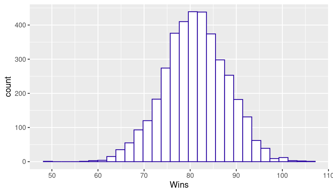
One expects these average teams to win about 81 games. But what is surprising is the variability in the win totals—average teams can regularly have win totals between 70 and 90, and it is possible (but not likely) to have a win total close to 100.
What is the relationship between a team’s talent and its post-season success? Consider first the relationship between a team’s talent (variable Talent) and winning the league (the variable Winner.Lg). Since Winner.Lg is a binary (0 or 1) variable, a common approach for representing this relationship is a logistic model; this is a generalization of the usual regression model where the response variable is binary instead of continuous. We use the glm() function with the family argument set to binomial to fit a logistic model; the output is stored in the variable fit1. In a similar fashion, we use a logistic model to model the relationship between winning the World Series (variable Winner.WS) and the talent; the output is in the variable fit2.
A logistic model has the form \[ p = \frac{\exp(a + b T)}{ 1 + \exp(a + b T)}, \] where \(T\) is a team’s talent, \((a, b)\) are the regression coefficients, and \(p\) is the probability of the event.
In the following code, we generate a vector of plausible values of a team’s talent and store them in the vector talent_values. We then compute fitted probabilities of winning the pennant and winning the World Series using the predict() function. (The type = "response" argument will map values of \(a + b T\) to the probability scale.) Then we construct a graph of talent against probability using the geom_line() function where the color of the line corresponds to the type of achievement. The completed graph is displayed in Figure 9.3.
tdf <- tibble(
  Talent =  seq(-0.4, 0.4, length.out = 100)
)
tdf |>
  mutate(
    Pennant = predict(fit1, newdata = tdf, type = "response"),
    `World Series` = predict(fit2, newdata = tdf, type = "response")
  ) |>
  pivot_longer(
    cols = -Talent,
    names_to = "Outcome",
    values_to = "Probability"
  ) |>
  ggplot(aes(Talent, Probability, color = Outcome)) +
  geom_line() + ylim(0, 1) +
  scale_color_manual(values = crc_fc)
As expected, the chance of a team winning the pennant (blue line) increases as a function of the talent. An average team with \(T = 0\) has only a small chance of winning the pennant; an excellent team with a talent close to 0.4 has about a 60% chance of winning the pennant. The probabilities of winning the World Series (represented by a red line) are substantially smaller than the chances of winning the pennant. For example, this excellent (\(T = 0.4\)) team has only about a 35% chance of winning the World Series. In fact, it can be demonstrated that the team winning the World Series is likely not to be the team with the best talent (largest value of \(T\)).
9.4 Further Reading
A general description of the Markov chain probability model is contained in Kemeny and Snell (1960). Pankin (1987) and Bukiet, Harold, and Palacios (1997) illustrate the use of Markov chains to model baseball. Chapter 9 of Albert (2017) gives an introductory description of Markov chains and illustrates the construction and use of the transition matrix using 1987 season data. The Bradley-Terry model (Bradley and Terry 1952) is a popular statistical model for paired comparisons. Chapter 9 of Albert and Bennett (2003) describes the application of the Bradley-Terry model for baseball team competition. The use of R in simulation is introduced in Chapter 11 of Albert and Rizzo (2012). Lopez, Matthews, and Baumer (2018) use a Bradley-Terry state space model to address the question of how often the best teams win.
9.5 Exercises
1. A Simple Markov Chain
Suppose one is interested only in the number of outs in an inning. There are four possible states in an inning (0 outs, 1 out, 2 outs, and 3 outs) and you move between these states in each plate appearance. Suppose at each PA, the chance of not increasing the number of outs is 0.3, and the probability of increasing the outs by one is 0.7. The following R code puts the transition probabilities of this Markov chain in a matrix P.
- If one multiplies the matrix
Pby itselfPto obtain the matrixP2:
P2 <- P %*% PThe first row of P2 gives the probabilities of moving from 0 outs to each of the four states after two plate appearances. Compute P2. Based on this computation, find the probability of moving from 0 outs to 1 out after two plate appearances.
- The fundamental matrix
Nis computed as
The first row gives the average number of PAs at 0 out, 1 out, and 2 outs in an inning. Compute N and find the average number of PAs in one inning in this model.
2. A Simple Markov Chain, Continued
The following function simulate_half_inning() will simulate the number of plate appearances in a single half-inning of the Markov chain model described in Exercise 1 where the input P is the transition probability matrix.
Use the
map()function to simulate 1000 half-innings of this Markov chain and store the lengths of these simulated innings in the vectorlengths.Using this simulated output, find the probability that a half-inning contains exactly four plate appearances.
Use the simulated output to find the average number of PAs in a half-inning. Compare your answer with the exact answer in Exercise 1, part (b).
3. Simulating a Half Inning
In Section 9.2.4, the expected number of runs as calculated for each one of the 24 possible runners-outs situations using data from the 2016 season. To see how these values can change across seasons, download play-by-play data from Retrosheet for the 1968 season, construct the probability transition matrix, simulate 10,000 half-innings from each of the 24 situations, and compute the run expectancy matrix. Compare this 1968 run expectancy matrix with the one computed using 2016 data.
4. Simulating the 1950 Season
Suppose you are interested in simulating the 1950 regular season for the National League. In this season, the team abbreviations were “PHI”, “BRO”, “NYG”, “BSN”, “STL”, “CIN”, “CHC”, and “PIT” and each team played every other team 22 games (11 games at each park).
Using the function
make_schedule(), construct the schedule of games for this NL season.Suppose the team talents follow a normal distribution with mean 0 and standard deviation 0.25. Using the Bradley-Terry model, assign home win probabilities for all games on the schedule.
Use the
rbinom()function to simulate the outcomes of all 616 games of the NL 1950 season.Compute the number of season wins for all teams in your simulation.
5. Simulating the 1950 Season, Continued
Write a function to perform the simulation scheme described in Exercise 4. Have the function return the team with the largest talent and the team with the most wins. (If there is a tie for the league pennant, have the function return one of the best teams at random.)
Repeat this simulation for 1000 seasons, collecting the most talented team and the most successful team for all seasons.
Based on your simulations, what is the chance that the most talented team wins the pennant?
6. Simulating the World Series
Write a function to simulate a World Series. The input is the probability
pthat the AL team will defeat the NL team in a single game.Suppose an AL team with talent \(0.40\) plays a NL team with talent \(0.25\). Using the Bradley-Terry model, determine the probability
pthat the AL wins a game.Using the value of
pdetermined in part (b), simulate 1000 World Series and find the probability the AL team wins the World Series.Repeat parts (b) and (c) for AL and NL teams who have the same talents.
This is often known as the memoryless property.↩︎